


Scatter Plots - R Base Graphs
Previously, we described the essentials of R programming and provided quick start guides for importing data into R.
Pleleminary tasks
Launch RStudio as described here: Running RStudio and setting up your working directory
Prepare your data as described here: Best practices for preparing your data and save it in an external .txt tab or .csv files
Import your data into R as described here: Fast reading of data from txt|csv files into R: readr package.
Here, we’ll use the R built-in mtcars data set.
R base scatter plot: plot()
x <- mtcars$wt
y <- mtcars$mpg
# Plot with main and axis titles
# Change point shape (pch = 19) and remove frame.
plot(x, y, main = "Main title",
     xlab = "X axis title", ylab = "Y axis title",
     pch = 19, frame = FALSE)
# Add regression line
plot(x, y, main = "Main title",
     xlab = "X axis title", ylab = "Y axis title",
     pch = 19, frame = FALSE)
abline(lm(y ~ x, data = mtcars), col = "blue")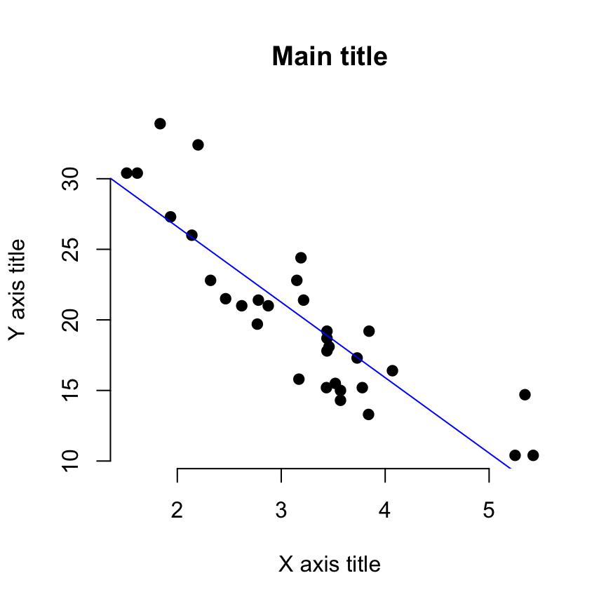
# Add loess fit
plot(x, y, main = "Main title",
     xlab = "X axis title", ylab = "Y axis title",
     pch = 19, frame = FALSE)
lines(lowess(x, y), col = "blue")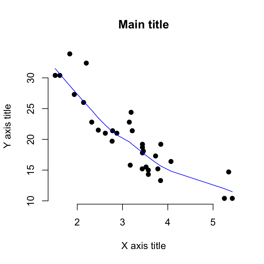
Enhanced scatter plots: car::scatterplot()
The function scatterplot() [in car package] makes enhanced scatter plots, with box plots in the margins, a non-parametric regression smooth, smoothed conditional spread, outlier identification, and a regression line, …
- Install car package:
install.packages("car")- Use scatterplot() function:
library("car")
scatterplot(wt ~ mpg, data = mtcars)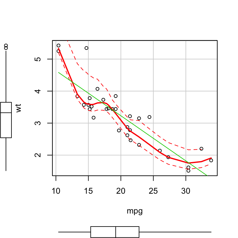
The plot contains:
- the points
- the regression line (in green)
- the smoothed conditional spread (in red dashed line)
- the non-parametric regression smooth (solid line, red)
# Suppress the smoother and frame
scatterplot(wt ~ mpg, data = mtcars,
            smoother = FALSE, grid = FALSE, frame = FALSE)
# Scatter plot by groups ("cyl")
scatterplot(wt ~ mpg | cyl, data = mtcars,
            smoother = FALSE, grid = FALSE, frame = FALSE)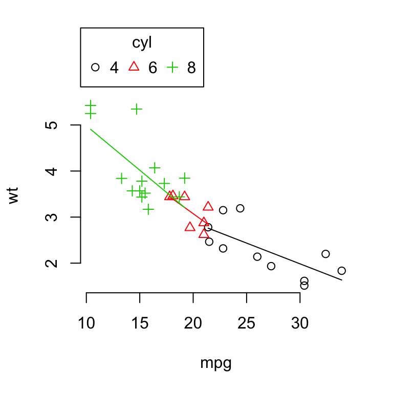
It’s also possible to add labels using the following arguments:
- labels: a vector of point labels
- id.n, id.cex, id.col: Arguments for labeling points specifying the number, the size and the color of points to be labelled.
# Add labels
scatterplot(wt ~ mpg, data = mtcars,
            smoother = FALSE, grid = FALSE, frame = FALSE,
            labels = rownames(mtcars), id.n = nrow(mtcars),
            id.cex = 0.7, id.col = "steelblue",
            ellipse = TRUE)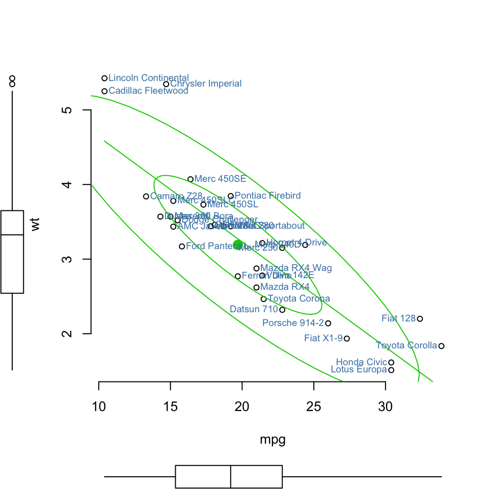
##           Mazda RX4       Mazda RX4 Wag          Datsun 710      Hornet 4 Drive   Hornet Sportabout             Valiant
##                   1                   2                   3                   4                   5                   6
##          Duster 360           Merc 240D            Merc 230            Merc 280           Merc 280C          Merc 450SE
##                   7                   8                   9                  10                  11                  12
##          Merc 450SL         Merc 450SLC  Cadillac Fleetwood Lincoln Continental   Chrysler Imperial            Fiat 128
##                  13                  14                  15                  16                  17                  18
##         Honda Civic      Toyota Corolla       Toyota Corona    Dodge Challenger         AMC Javelin          Camaro Z28
##                  19                  20                  21                  22                  23                  24
##    Pontiac Firebird           Fiat X1-9       Porsche 914-2        Lotus Europa      Ford Pantera L        Ferrari Dino
##                  25                  26                  27                  28                  29                  30
##       Maserati Bora          Volvo 142E
##                  31                  32
Other arguments can be used such as:
- log to produce log axes. Allowed values are log = “x”, log = “y” or log = “xy”
- boxplots: Allowed values are:
- “x”: a box plot for x is drawn below the plot
- “y”: a box plot for y is drawn to the left of the plot
- “xy”: both box plots are drawn
- “” or FALSE to suppress both box plots.
- ellipse: if TRUE data-concentration ellipses are plotted.
3D scatter plots
To plot a 3D scatterplot the function scatterplot3D [in scatterplot3D package can be used].
The following R code plots a 3D scatter plot using iris data set.
head(iris)## Sepal.Length Sepal.Width Petal.Length Petal.Width Species
## 1 5.1 3.5 1.4 0.2 setosa
## 2 4.9 3.0 1.4 0.2 setosa
## 3 4.7 3.2 1.3 0.2 setosa
## 4 4.6 3.1 1.5 0.2 setosa
## 5 5.0 3.6 1.4 0.2 setosa
## 6 5.4 3.9 1.7 0.4 setosa# Prepare the data set
x <- iris$Sepal.Length
y <- iris$Sepal.Width
z <- iris$Petal.Length
grps <- as.factor(iris$Species)
# Plot
library(scatterplot3d)
scatterplot3d(x, y, z, pch = 16)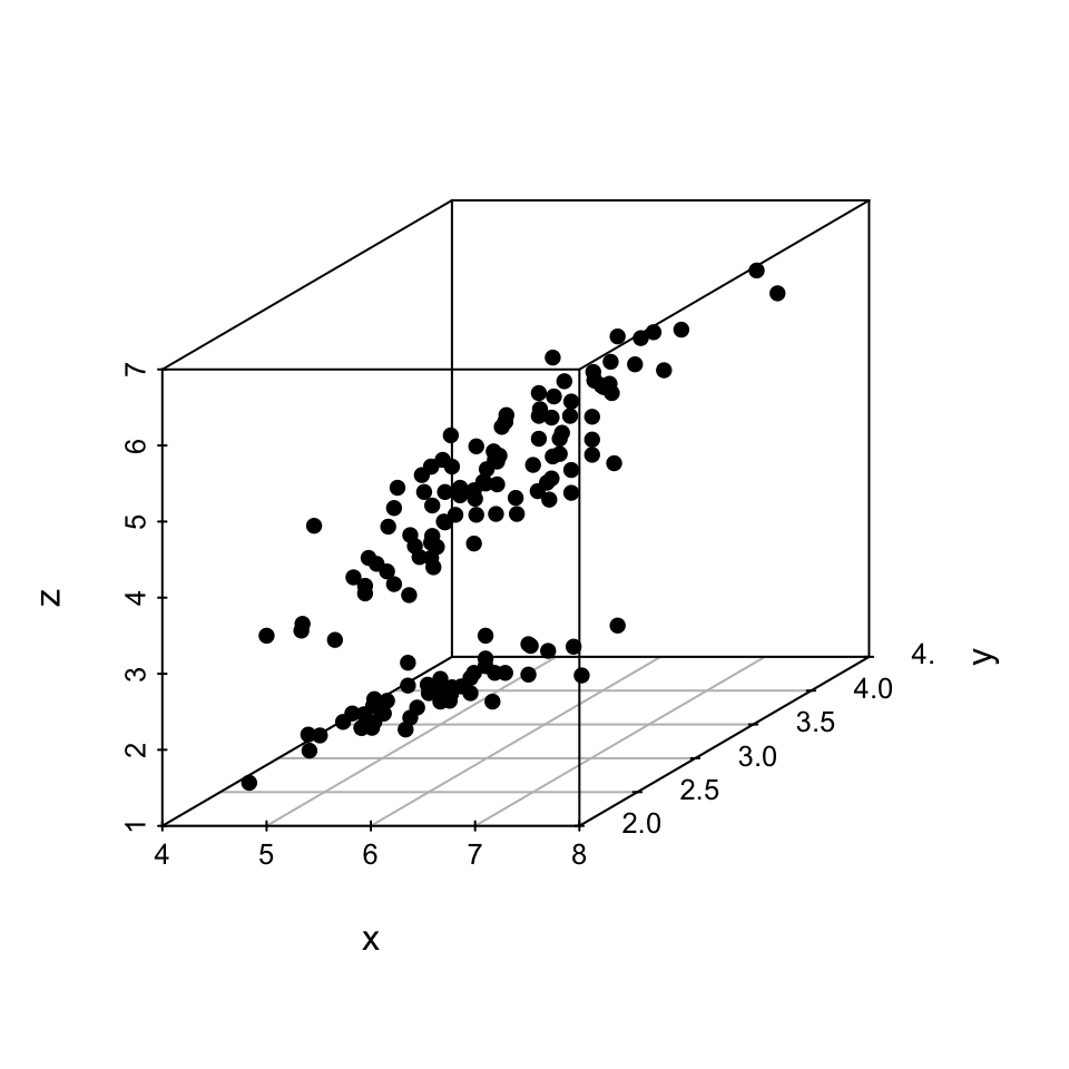
# Change color by groups
# add grids and remove the box around the plot
# Change axis labels: xlab, ylab and zlab
colors <- c("#999999", "#E69F00", "#56B4E9")
scatterplot3d(x, y, z, pch = 16, color = colors[grps],
              grid = TRUE, box = FALSE, xlab = "Sepal length",
              ylab = "Sepal width", zlab = "Petal length")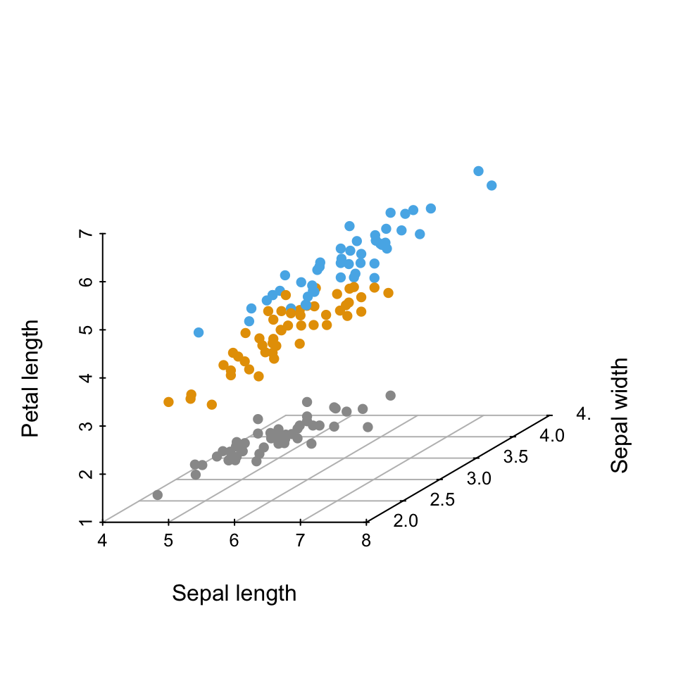
- Read more about static and interactive 3D scatter plot:
Summary
Create a scatter plot:
- Using R base function:
with(mtcars, plot(wt, mpg, frame = FALSE))- Using car package:
car::scatterplot(wt ~ mpg, data = mtcars,
smoother = FALSE, grid = FALSE)- 3D scatter plot:
library(scatterplot3d)
with(iris,
     scatterplot3d(x = Sepal.Length, y = Sepal.Width,
                   z = Petal.Length, pch = 16,
                   grid = TRUE, box = FALSE)
)See also
Infos
This analysis has been performed using R statistical software (ver. 3.2.4).
Show me some love with the like buttons below... Thank you and please don't forget to share and comment below!!
Montrez-moi un peu d'amour avec les like ci-dessous ... Merci et n'oubliez pas, s'il vous plaît, de partager et de commenter ci-dessous!
Recommended for You!


Recommended for you
This section contains the best data science and self-development resources to help you on your path.
Books - Data Science
Our Books
- Practical Guide to Cluster Analysis in R by A. Kassambara (Datanovia)
- Practical Guide To Principal Component Methods in R by A. Kassambara (Datanovia)
- Machine Learning Essentials: Practical Guide in R by A. Kassambara (Datanovia)
- R Graphics Essentials for Great Data Visualization by A. Kassambara (Datanovia)
- GGPlot2 Essentials for Great Data Visualization in R by A. Kassambara (Datanovia)
- Network Analysis and Visualization in R by A. Kassambara (Datanovia)
- Practical Statistics in R for Comparing Groups: Numerical Variables by A. Kassambara (Datanovia)
- Inter-Rater Reliability Essentials: Practical Guide in R by A. Kassambara (Datanovia)
Others
- R for Data Science: Import, Tidy, Transform, Visualize, and Model Data by Hadley Wickham & Garrett Grolemund
- Hands-On Machine Learning with Scikit-Learn, Keras, and TensorFlow: Concepts, Tools, and Techniques to Build Intelligent Systems by Aurelien Géron
- Practical Statistics for Data Scientists: 50 Essential Concepts by Peter Bruce & Andrew Bruce
- Hands-On Programming with R: Write Your Own Functions And Simulations by Garrett Grolemund & Hadley Wickham
- An Introduction to Statistical Learning: with Applications in R by Gareth James et al.
- Deep Learning with R by François Chollet & J.J. Allaire
- Deep Learning with Python by François Chollet
Click to follow us on Facebook :
Comment this article by clicking on "Discussion" button (top-right position of this page)