


survminer 0.2.4
I’m very pleased to announce survminer 0.2.4. It comes with many new features and minor changes.
Install survminer with:
install.packages("survminer")To load the package, type this:
library(survminer)New features
- New function
surv_summary()for creating data frame containing a nice summary of survival curves (#64). - It’s possible now to facet the output of
ggsurvplot()by one or more factors (#64). - Now,
ggsurvplot()can be used to plot cox model (#67). - New functions added for determining and visualizing the optimal cutpoint of continuous variables for survival analyses:
surv_cutpoint(): Determine the optimal cutpoint for each variable using ‘maxstat’. Methods defined for surv_cutpoint object are summary(), print() and plot().surv_categorize(): Divide each variable values based on the cutpoint returned bysurv_cutpoint()(#41).
- New argument ‘ncensor.plot’ added to
ggsurvplot(). A logical value. If TRUE, the number of censored subjects at time t is plotted. Default is FALSE (#18).
Minor changes
- New argument ‘conf.int.style’ added in
ggsurvplot()for changing the style of confidence interval bands. - Now,
ggsurvplot()plots a stepped confidence interval when conf.int = TRUE (#65). ggsurvplot()updated for compatibility with the future version of ggplot2 (v2.2.0) (#68)- ylab is now automatically adapted according to the value of the argument
fun. For example, if fun = “event”, then ylab will be “Cumulative event”. - In
ggsurvplot(), linetypes can now be adjusted by variables used to fit survival curves (#46) - In
ggsurvplot(), the argument risk.table can be either a logical value (TRUE|FALSE) or a string (“absolute”, “percentage”). If risk.table = “absolute”,ggsurvplot()displays the absolute number of subjects at risk. If risk.table = “percentage”, the percentage at risk is displayed. Use “abs_pct” to show both the absolute number and the percentage of subjects at risk. (#70). - New argument surv.median.line in
ggsurvplot(): character vector for drawing a horizontal/vertical line at median (50%) survival. Allowed values include one of c(“none”, “hv”, “h”, “v”). v: vertical, h:horizontal (#61). - Now, the default theme of ggcoxdiagnostics() is ggplot2::theme_bw().
Summary of survival curves
Compared to the default summary() function, the surv_summary() function [in survminer] creates a data frame containing a nice summary from survfit results.
# Fit survival curves
require("survival")
fit <- survfit(Surv(time, status) ~ sex, data = lung)
# Summarize
library("survminer")
res.sum <- surv_summary(fit)
head(res.sum)
## time n.risk n.event n.censor surv std.err upper lower
## 1 11 138 3 0 0.9782609 0.01268978 1.0000000 0.9542301
## 2 12 135 1 0 0.9710145 0.01470747 0.9994124 0.9434235
## 3 13 134 2 0 0.9565217 0.01814885 0.9911586 0.9230952
## 4 15 132 1 0 0.9492754 0.01967768 0.9866017 0.9133612
## 5 26 131 1 0 0.9420290 0.02111708 0.9818365 0.9038355
## 6 30 130 1 0 0.9347826 0.02248469 0.9768989 0.8944820
## strata sex
## 1 sex=1 1
## 2 sex=1 1
## 3 sex=1 1
## 4 sex=1 1
## 5 sex=1 1
## 6 sex=1 1# Information about the survival curves
attr(res.sum, "table")## records n.max n.start events *rmean *se(rmean) median 0.95LCL
## sex=1 138 138 138 112 325.0663 22.59845 270 212
## sex=2 90 90 90 53 458.2757 33.78530 426 348
## 0.95UCL
## sex=1 310
## sex=2 550Plot survival curves
ggsurvplot(
   fit,                     # survfit object with calculated statistics.
   pval = TRUE,             # show p-value of log-rank test.
   conf.int = TRUE,         # show confidence intervals for
                            # point estimaes of survival curves.
   #conf.int.style = "step",  # customize style of confidence intervals
   xlab = "Time in days",   # customize X axis label.
   break.time.by = 200,     # break X axis in time intervals by 200.
   ggtheme = theme_light(), # customize plot and risk table with a theme.
   risk.table = "abs_pct",  # absolute number and percentage at risk.
  risk.table.y.text.col = T,# colour risk table text annotations.
  risk.table.y.text = FALSE,# show bars instead of names in text annotations
                            # in legend of risk table.
  ncensor.plot = TRUE,      # plot the number of censored subjects at time t
  surv.median.line = "hv",  # add the median survival pointer.
  legend.labs =
    c("Male", "Female"),    # change legend labels.
  palette =
    c("#E7B800", "#2E9FDF") # custom color palettes.
)
survminer
Determine the optimal cutpoint for continuous variables
The survminer package determines the optimal cutpoint for one or multiple continuous variables at once, using the maximally selected rank statistics from the ‘maxstat’ R package. To learn more, read this: M. Kosiński. R-ADDICT November 2016. Determine optimal cutpoints for numerical variables in survival plots.
Here, we’ll use the myeloma data sets [in the survminer package]. It contains survival data and some gene expression data obtained from multiple myeloma patients.
# 0. Load some data
data(myeloma)
head(myeloma[, 1:8])
## molecular_group chr1q21_status treatment event time CCND1
## GSM50986 Cyclin D-1 3 copies TT2 0 69.24 9908.4
## GSM50988 Cyclin D-2 2 copies TT2 0 66.43 16698.8
## GSM50989 MMSET 2 copies TT2 0 66.50 294.5
## GSM50990 MMSET 3 copies TT2 1 42.67 241.9
## GSM50991 MAF TT2 0 65.00 472.6
## GSM50992 Hyperdiploid 2 copies TT2 0 65.20 664.1
## CRIM1 DEPDC1
## GSM50986 420.9 523.5
## GSM50988 52.0 21.1
## GSM50989 617.9 192.9
## GSM50990 11.9 184.7
## GSM50991 38.8 212.0
## GSM50992 16.9 341.6 # 1. Determine the optimal cutpoint of variables
res.cut <- surv_cutpoint(myeloma, time = "time", event = "event",
variables = c("DEPDC1", "WHSC1", "CRIM1"))
summary(res.cut)## cutpoint statistic
## DEPDC1 279.8 4.275452
## WHSC1 3205.6 3.361330
## CRIM1 82.3 1.968317# 2. Plot cutpoint for DEPDC1
# palette = "npg" (nature publishing group), see ?ggpubr::ggpar
plot(res.cut, "DEPDC1", palette = "npg")## $DEPDC1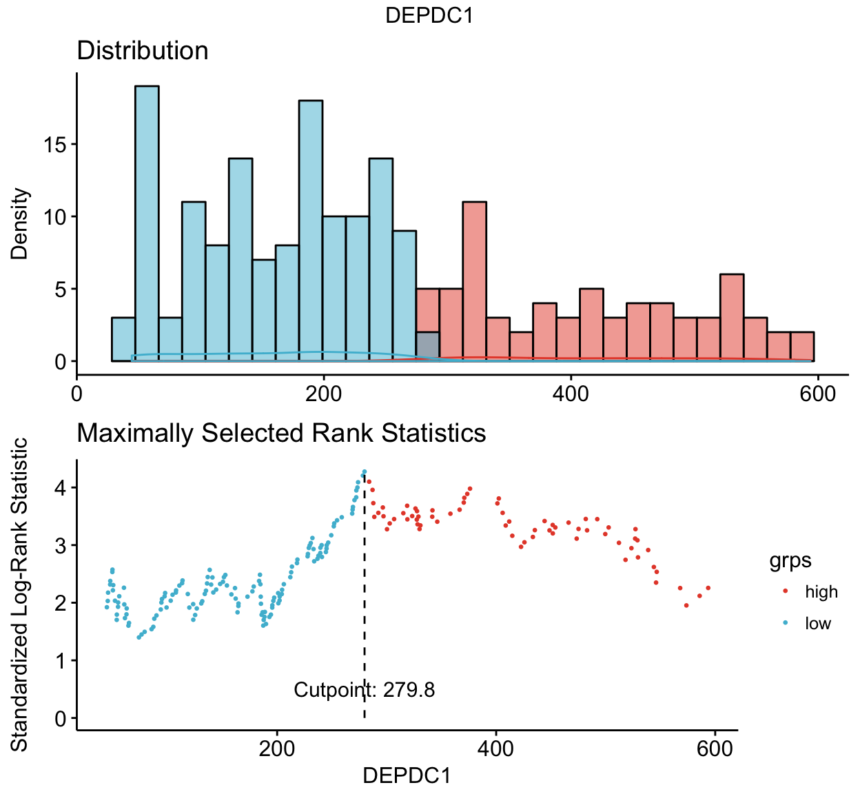
survminer
# 3. Categorize variables
res.cat <- surv_categorize(res.cut)
head(res.cat)
## time event DEPDC1 WHSC1 CRIM1
## GSM50986 69.24 0 high low high
## GSM50988 66.43 0 low low low
## GSM50989 66.50 0 low high high
## GSM50990 42.67 1 low high low
## GSM50991 65.00 0 low low low
## GSM50992 65.20 0 high low low# 4. Fit survival curves and visualize
library("survival")
fit <- survfit(Surv(time, event) ~DEPDC1, data = res.cat)
ggsurvplot(fit, risk.table = TRUE, conf.int = TRUE)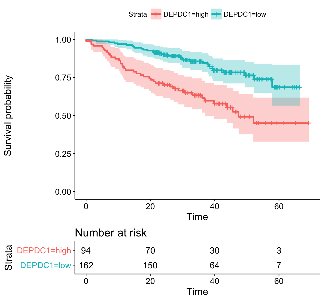
survminer
Facet the output of ggsurvplot()
In this section, we’ll compute survival curves using the combination of multiple factors. Next, we’ll factet the output of ggsurvplot() by a combination of factors
- Fit (complex) survival curves using colon data sets
require("survival")
fit2 <- survfit( Surv(time, status) ~ sex + rx + adhere,
data = colon )- Visualize the output using survminer
ggsurv <- ggsurvplot(fit2, fun = "event", conf.int = TRUE,
  risk.table = TRUE, risk.table.col="strata",
  ggtheme = theme_bw())
ggsurv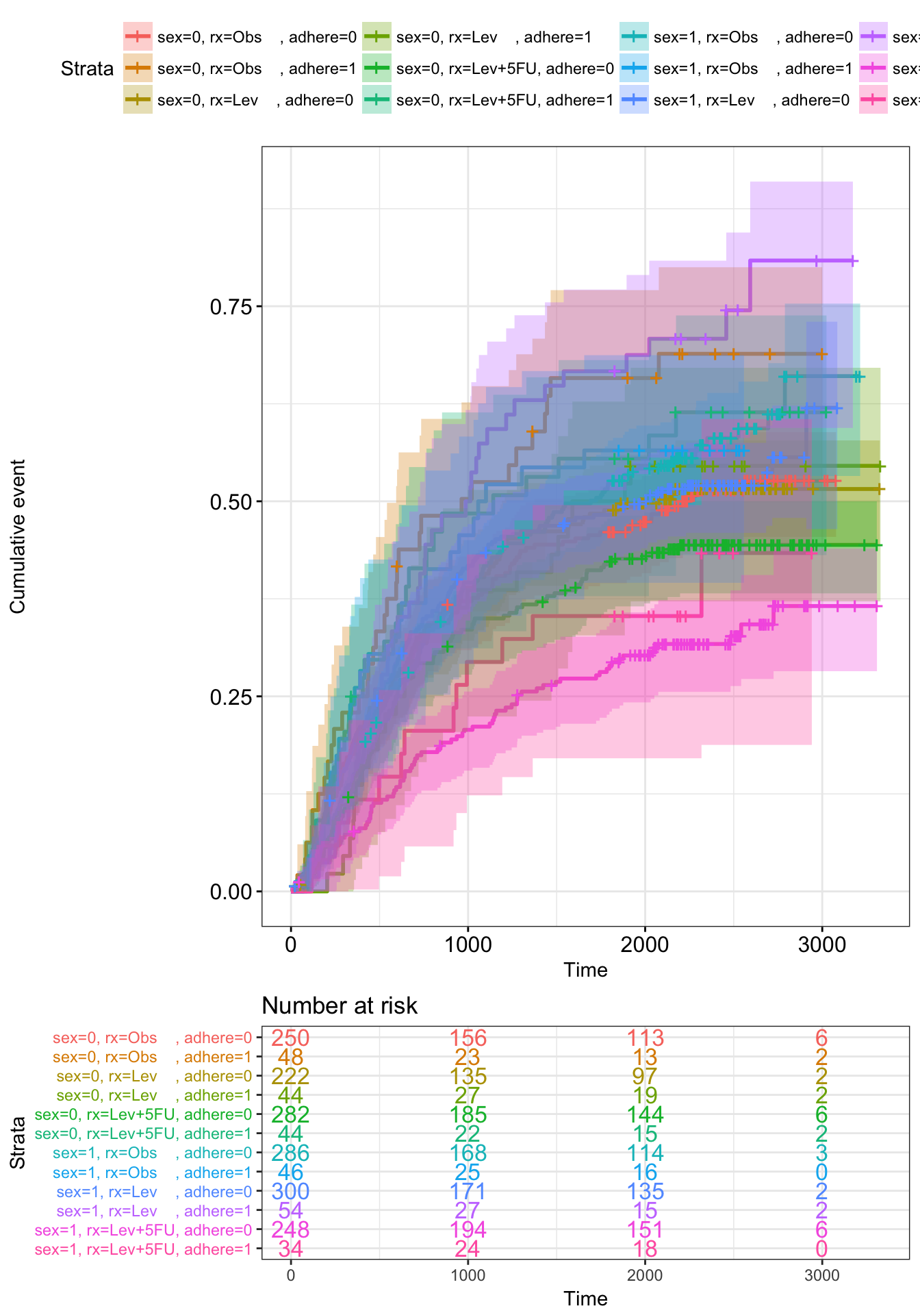
survminer
- Faceting survival curves. The plot below shows survival curves by the sex variable faceted according to the values of rx & adhere.
curv_facet <- ggsurv$plot + facet_grid(rx ~ adhere)
curv_facet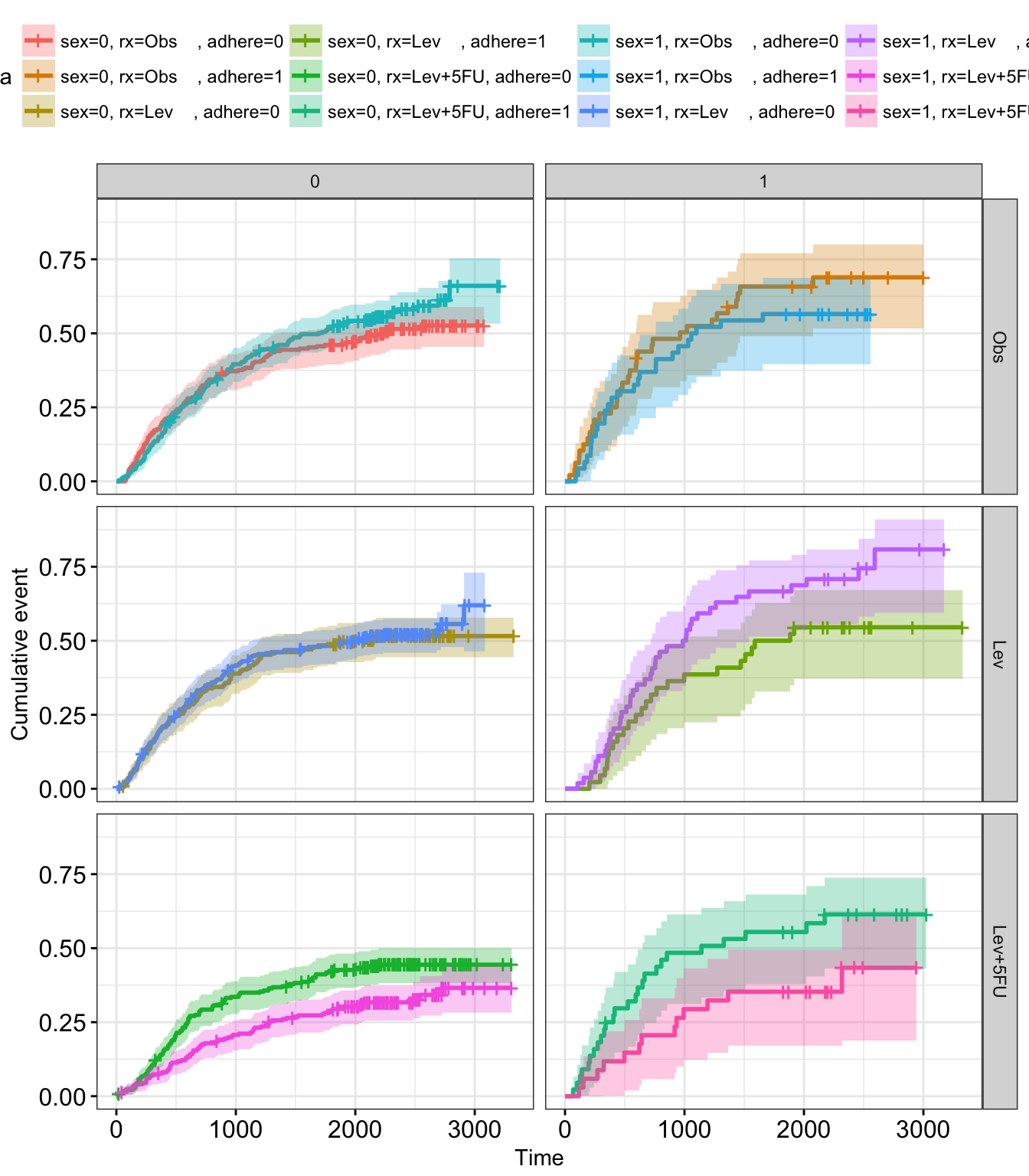
survminer
- Facetting risk tables: Generate risk table for each facet plot item
ggsurv$table + facet_grid(rx ~ adhere, scales = "free")+
 theme(legend.position = "none")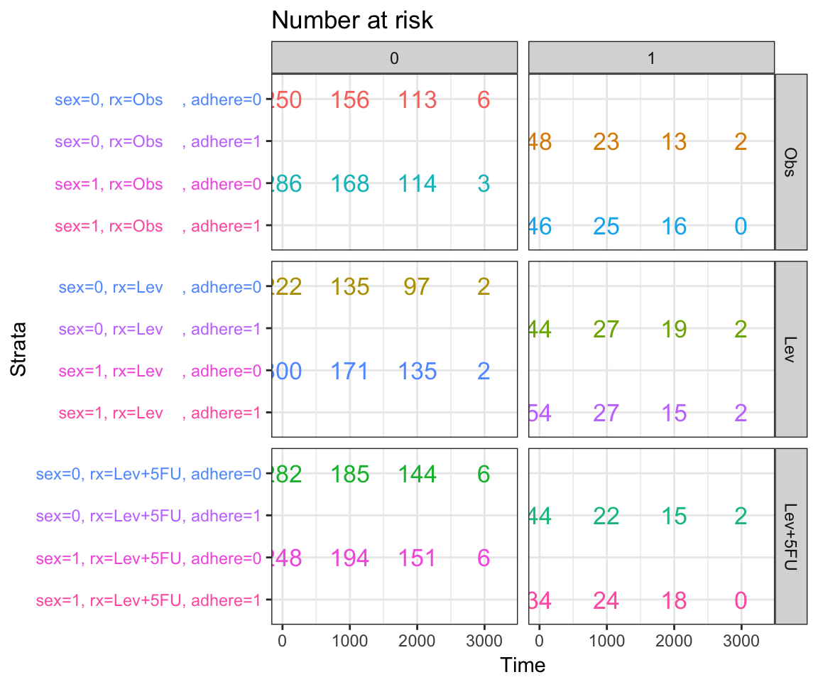
survminer
- Generate risk table for each facet columns
tbl_facet <- ggsurv$table + facet_grid(.~ adhere, scales = "free")
tbl_facet + theme(legend.position = "none")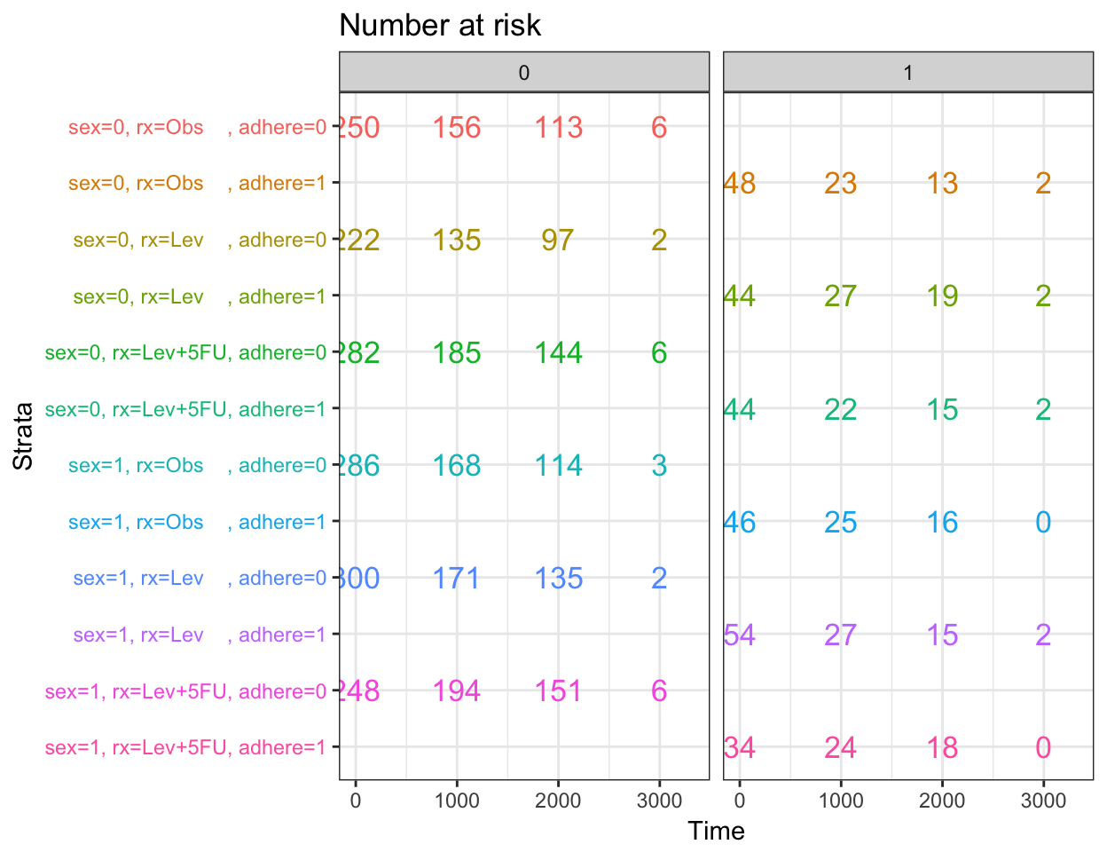
survminer
# Arrange faceted survival curves and risk tables
g2 <- ggplotGrob(curv_facet)
g3 <- ggplotGrob(tbl_facet)
min_ncol <- min(ncol(g2), ncol(g3))
g <- gridExtra::rbind.gtable(g2[, 1:min_ncol], g3[, 1:min_ncol], size="last")
g$widths <- grid::unit.pmax(g2$widths, g3$widths)
grid::grid.newpage()
grid::grid.draw(g)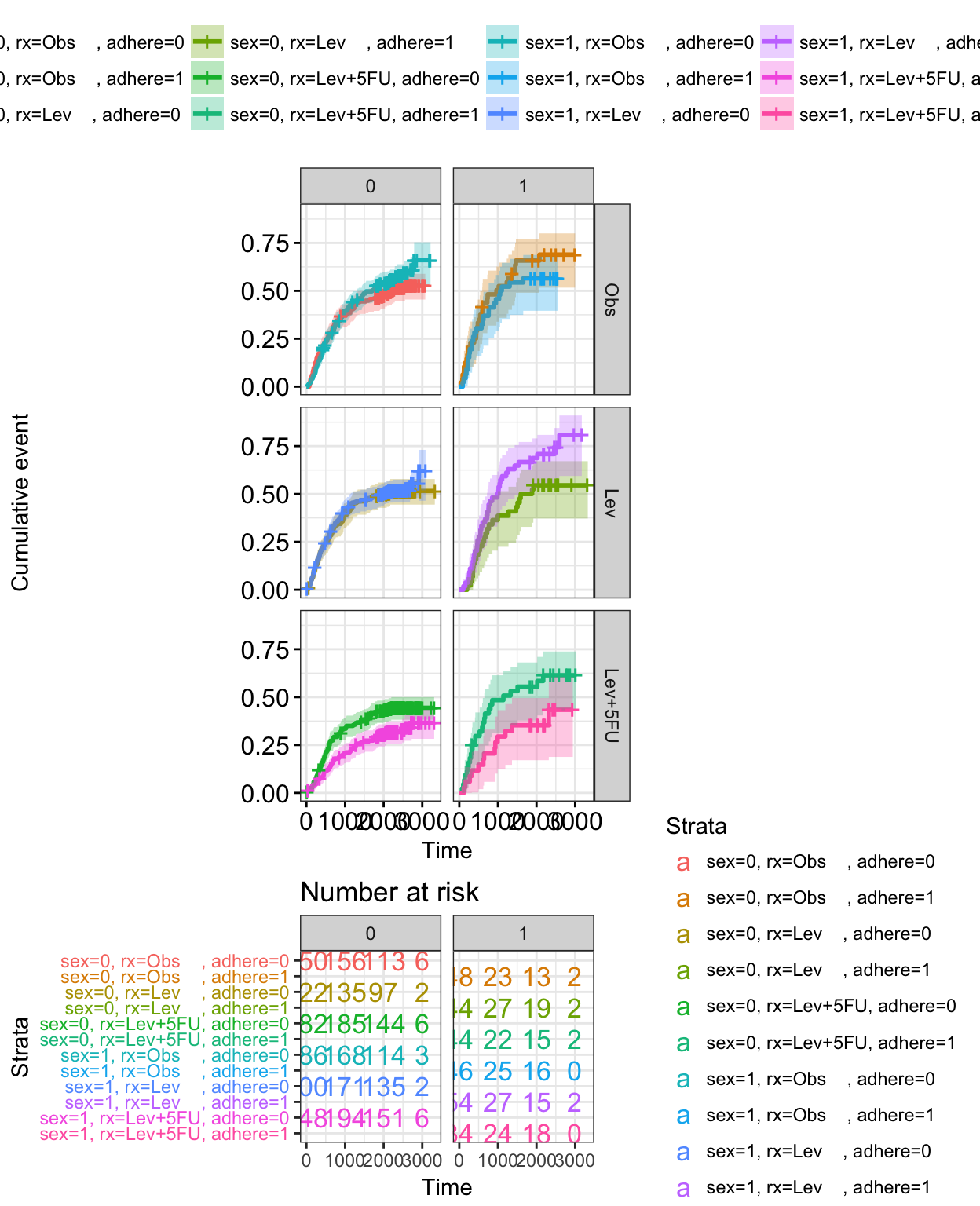
survminer
Infos
This analysis has been performed using R software (ver. 3.3.2).
Show me some love with the like buttons below... Thank you and please don't forget to share and comment below!!
Montrez-moi un peu d'amour avec les like ci-dessous ... Merci et n'oubliez pas, s'il vous plaît, de partager et de commenter ci-dessous!
Recommended for You!


Recommended for you
This section contains the best data science and self-development resources to help you on your path.
Books - Data Science
Our Books
- Practical Guide to Cluster Analysis in R by A. Kassambara (Datanovia)
- Practical Guide To Principal Component Methods in R by A. Kassambara (Datanovia)
- Machine Learning Essentials: Practical Guide in R by A. Kassambara (Datanovia)
- R Graphics Essentials for Great Data Visualization by A. Kassambara (Datanovia)
- GGPlot2 Essentials for Great Data Visualization in R by A. Kassambara (Datanovia)
- Network Analysis and Visualization in R by A. Kassambara (Datanovia)
- Practical Statistics in R for Comparing Groups: Numerical Variables by A. Kassambara (Datanovia)
- Inter-Rater Reliability Essentials: Practical Guide in R by A. Kassambara (Datanovia)
Others
- R for Data Science: Import, Tidy, Transform, Visualize, and Model Data by Hadley Wickham & Garrett Grolemund
- Hands-On Machine Learning with Scikit-Learn, Keras, and TensorFlow: Concepts, Tools, and Techniques to Build Intelligent Systems by Aurelien Géron
- Practical Statistics for Data Scientists: 50 Essential Concepts by Peter Bruce & Andrew Bruce
- Hands-On Programming with R: Write Your Own Functions And Simulations by Garrett Grolemund & Hadley Wickham
- An Introduction to Statistical Learning: with Applications in R by Gareth James et al.
- Deep Learning with R by François Chollet & J.J. Allaire
- Deep Learning with Python by François Chollet
Click to follow us on Facebook :
Comment this article by clicking on "Discussion" button (top-right position of this page)