


Normality Test in R
Many of statistical tests including correlation, regression, t-test, and analysis of variance (ANOVA) assume some certain characteristics about the data. They require the data to follow a normal distribution or Gaussian distribution. These tests are called parametric tests, because their validity depends on the distribution of the data.
Normality and the other assumptions made by these tests should be taken seriously to draw reliable interpretation and conclusions of the research.
Before using a parametric test, we should perform some preleminary tests to make sure that the test assumptions are met. In the situations where the assumptions are violated, non-paramatric tests are recommended.
Here, we’ll describe how to check the normality of the data by visual inspection and by significance tests.
Install required R packages
- dplyr for data manipulation
install.packages("dplyr")- ggpubr for an easy ggplot2-based data visualization
- Install the latest version from GitHub as follow:
# Install
if(!require(devtools)) install.packages("devtools")
devtools::install_github("kassambara/ggpubr")- Or, install from CRAN as follow:
install.packages("ggpubr")Load required R packages
library("dplyr")
library("ggpubr")
Import your data into R
Prepare your data as specified here: Best practices for preparing your data set for R
Save your data in an external .txt tab or .csv files
Import your data into R as follow:
# If .txt tab file, use this
my_data <- read.delim(file.choose())
# Or, if .csv file, use this
my_data <- read.csv(file.choose())
Here, we’ll use the built-in R data set named ToothGrowth.
# Store the data in the variable my_data
my_data <- ToothGrowth
Check your data
We start by displaying a random sample of 10 rows using the function sample_n()[in dplyr package].
Show 10 random rows:
set.seed(1234)
dplyr::sample_n(my_data, 10)
len supp dose
7 11.2 VC 0.5
37 8.2 OJ 0.5
36 10.0 OJ 0.5
58 27.3 OJ 2.0
49 14.5 OJ 1.0
57 26.4 OJ 2.0
1 4.2 VC 0.5
13 15.2 VC 1.0
35 14.5 OJ 0.5
27 26.7 VC 2.0Assess the normality of the data in R
We want to test if the variable len (tooth length) is normally distributed.
Case of large sample sizes
If the sample size is large enough (n > 30), we can ignore the distribution of the data and use parametric tests.
The central limit theorem tells us that no matter what distribution things have, the sampling distribution tends to be normal if the sample is large enough (n > 30).
However, to be consistent, normality can be checked by visual inspection [normal plots (histogram), Q-Q plot (quantile-quantile plot)] or by significance tests].
Visual methods
Density plot and Q-Q plot can be used to check normality visually.
- Density plot: the density plot provides a visual judgment about whether the distribution is bell shaped.
library("ggpubr")
ggdensity(my_data$len,
          main = "Density plot of tooth length",
          xlab = "Tooth length")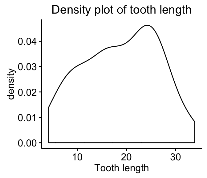
- Q-Q plot: Q-Q plot (or quantile-quantile plot) draws the correlation between a given sample and the normal distribution. A 45-degree reference line is also plotted.
library(ggpubr)
ggqqplot(my_data$len)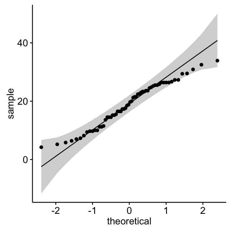
It’s also possible to use the function qqPlot() [in car package]:
library("car")
qqPlot(my_data$len)
As all the points fall approximately along this reference line, we can assume normality.
Normality test
Visual inspection, described in the previous section, is usually unreliable. It’s possible to use a significance test comparing the sample distribution to a normal one in order to ascertain whether data show or not a serious deviation from normality.
There are several methods for normality test such as Kolmogorov-Smirnov (K-S) normality test and Shapiro-Wilk’s test.
The null hypothesis of these tests is that “sample distribution is normal”. If the test is significant, the distribution is non-normal.
Shapiro-Wilk’s method is widely recommended for normality test and it provides better power than K-S. It is based on the correlation between the data and the corresponding normal scores.
Note that, normality test is sensitive to sample size. Small samples most often pass normality tests. Therefore, it’s important to combine visual inspection and significance test in order to take the right decision.
The R function shapiro.test() can be used to perform the Shapiro-Wilk test of normality for one variable (univariate):
shapiro.test(my_data$len)
    Shapiro-Wilk normality test
data:  my_data$len
W = 0.96743, p-value = 0.1091
From the output, the p-value > 0.05 implying that the distribution of the data are not significantly different from normal distribution. In other words, we can assume the normality.
Infos
This analysis has been performed using R software (ver. 3.2.4).
Show me some love with the like buttons below... Thank you and please don't forget to share and comment below!!
Montrez-moi un peu d'amour avec les like ci-dessous ... Merci et n'oubliez pas, s'il vous plaît, de partager et de commenter ci-dessous!
Recommended for You!


Recommended for you
This section contains the best data science and self-development resources to help you on your path.
Books - Data Science
Our Books
- Practical Guide to Cluster Analysis in R by A. Kassambara (Datanovia)
- Practical Guide To Principal Component Methods in R by A. Kassambara (Datanovia)
- Machine Learning Essentials: Practical Guide in R by A. Kassambara (Datanovia)
- R Graphics Essentials for Great Data Visualization by A. Kassambara (Datanovia)
- GGPlot2 Essentials for Great Data Visualization in R by A. Kassambara (Datanovia)
- Network Analysis and Visualization in R by A. Kassambara (Datanovia)
- Practical Statistics in R for Comparing Groups: Numerical Variables by A. Kassambara (Datanovia)
- Inter-Rater Reliability Essentials: Practical Guide in R by A. Kassambara (Datanovia)
Others
- R for Data Science: Import, Tidy, Transform, Visualize, and Model Data by Hadley Wickham & Garrett Grolemund
- Hands-On Machine Learning with Scikit-Learn, Keras, and TensorFlow: Concepts, Tools, and Techniques to Build Intelligent Systems by Aurelien Géron
- Practical Statistics for Data Scientists: 50 Essential Concepts by Peter Bruce & Andrew Bruce
- Hands-On Programming with R: Write Your Own Functions And Simulations by Garrett Grolemund & Hadley Wickham
- An Introduction to Statistical Learning: with Applications in R by Gareth James et al.
- Deep Learning with R by François Chollet & J.J. Allaire
- Deep Learning with Python by François Chollet
Click to follow us on Facebook :
Comment this article by clicking on "Discussion" button (top-right position of this page)