


Lattice Graphs
Previously, we described the essentials of R programming and provided quick start guides for importing data into R. We also showed how to visualize data using R base graphs.
Pleleminary tasks
Launch RStudio as described here: Running RStudio and setting up your working directory
Prepare your data as described here: Best practices for preparing your data and save it in an external .txt tab or .csv files
Import your data into R as described here: Fast reading of data from txt|csv files into R: readr package.
Briefly, if your data is saved in an external .txt tab or .csv files, use the following script to import the data into R:
# If .txt tab file use this:
my_data <- read.delim(file.choose())
# or if .csv file:
my_data <- read.csv(file.choose())
In the following sections, we’ll use R built-in data sets.
Installing and loading the lattice package
# Install
install.packages("lattice")
# Load
library("lattice")
Main functions in the lattice package
| Function | Description |
|---|---|
| xyplot() | Scatter plot |
| splom() | Scatter plot matrix |
| cloud() | 3D scatter plot |
| stripplot() | strip plots (1-D scatter plots) |
| bwplot() | Box plot |
| dotplot() | Dot plot |
| barchart() | bar chart |
| histogram() | Histogram |
| densityplot | Kernel density plot |
| qqmath() | Theoretical quantile plot |
| qq() | Two-sample quantile plot |
| contourplot() | 3D contour plot of surfaces |
| levelplot() | False color level plot of surfaces |
| parallel() | Parallel coordinates plot |
| wireframe() | 3D wireframe graph |
Note that, other functions (ecdfplot() and mapplot()) are available in the latticeExtra package.
xyplot(): Scatter plot
- R function: The R function xyplot() is used to produce bivariate scatter plots or time-series plots. The simplified format is as follow:
xyplot(y ~ x, data)- Data set: mtcars
my_data <- iris
head(my_data)
## Sepal.Length Sepal.Width Petal.Length Petal.Width Species
## 1 5.1 3.5 1.4 0.2 setosa
## 2 4.9 3.0 1.4 0.2 setosa
## 3 4.7 3.2 1.3 0.2 setosa
## 4 4.6 3.1 1.5 0.2 setosa
## 5 5.0 3.6 1.4 0.2 setosa
## 6 5.4 3.9 1.7 0.4 setosa- Basic scatter plot: y ~ x
# Default plot
xyplot(Sepal.Length ~ Petal.Length, data = my_data)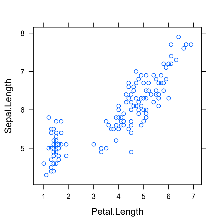
# Color by groups
xyplot(Sepal.Length ~ Petal.Length, group = Species,
       data = my_data, auto.key = TRUE)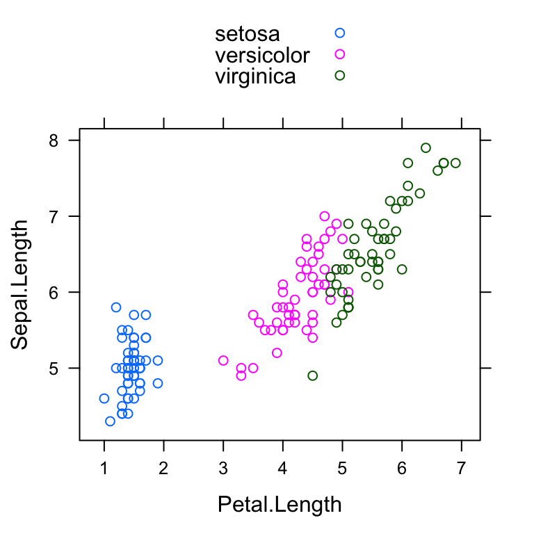
# Show points ("p"), grids ("g") and smoothing line
# Change xlab and ylab
xyplot(Sepal.Length ~ Petal.Length, data = my_data,
       type = c("p", "g", "smooth"),
       xlab = "Miles/(US) gallon", ylab = "Weight (1000 lbs)")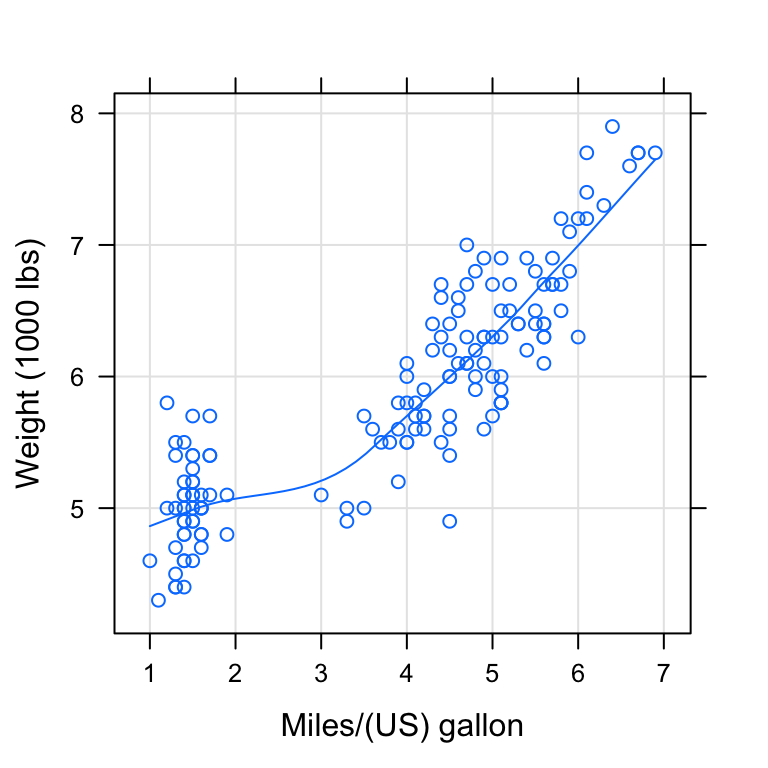
- Multiple panels by groups: y ~ x | group
xyplot(Sepal.Length ~ Petal.Length | Species,
       group = Species, data = my_data,
       type = c("p", "smooth"),
       scales = "free")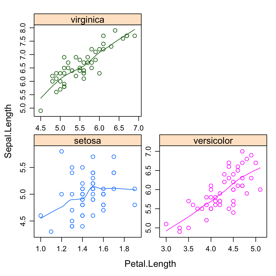
cloud(): 3D scatter plot
- Data set: iris
my_data <- iris
head(my_data)
## Sepal.Length Sepal.Width Petal.Length Petal.Width Species
## 1 5.1 3.5 1.4 0.2 setosa
## 2 4.9 3.0 1.4 0.2 setosa
## 3 4.7 3.2 1.3 0.2 setosa
## 4 4.6 3.1 1.5 0.2 setosa
## 5 5.0 3.6 1.4 0.2 setosa
## 6 5.4 3.9 1.7 0.4 setosa- Scatter 3D plot: z ~ x * y
# Basic 3D scatter plot
cloud(Sepal.Length ~ Sepal.Length * Petal.Width,
       data = iris)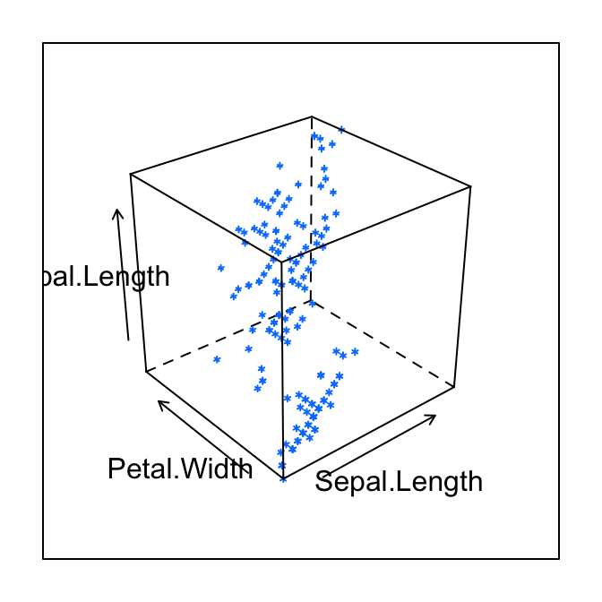
# Color by groups; auto.key = TRUE to show legend
cloud(Sepal.Length ~ Sepal.Length * Petal.Width,
       group = Species, data = iris,
       auto.key = TRUE)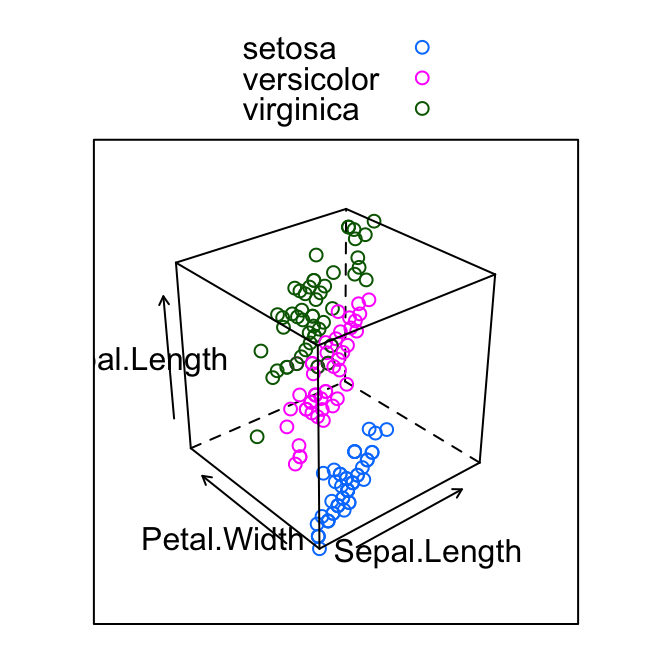
Box plot, Dot plot, Strip plot
- Data set: ToothGrowth
ToothGrowth$dose <- as.factor(ToothGrowth$dose)
head(ToothGrowth)
## len supp dose
## 1 4.2 VC 0.5
## 2 11.5 VC 0.5
## 3 7.3 VC 0.5
## 4 5.8 VC 0.5
## 5 6.4 VC 0.5
## 6 10.0 VC 0.5- Basic plot: Plot len by dose
# Basic box plot
bwplot(len ~ dose, data = ToothGrowth,
xlab = "Dose", ylab = "Length")
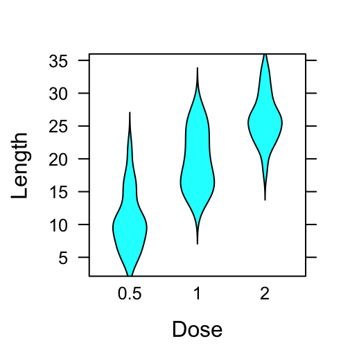
# Violin plot using panel = panel.violin
bwplot(len ~ dose, data = ToothGrowth,
panel = panel.violin,
xlab = "Dose", ylab = "Length")
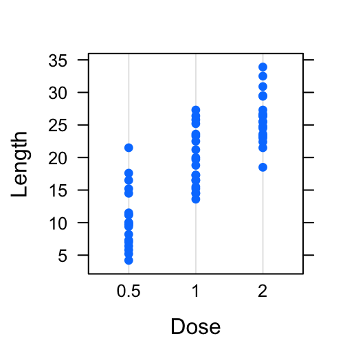
# Basic dot plot
dotplot(len ~ dose, data = ToothGrowth,
xlab = "Dose", ylab = "Length")
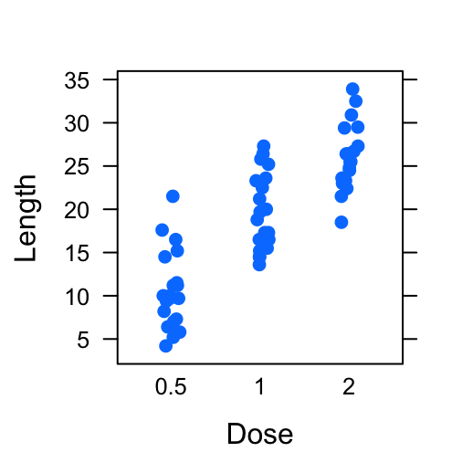
# Basic stip plot
stripplot(len ~ dose, data = ToothGrowth,
jitter.data = TRUE, pch = 19,
xlab = "Dose", ylab = "Length")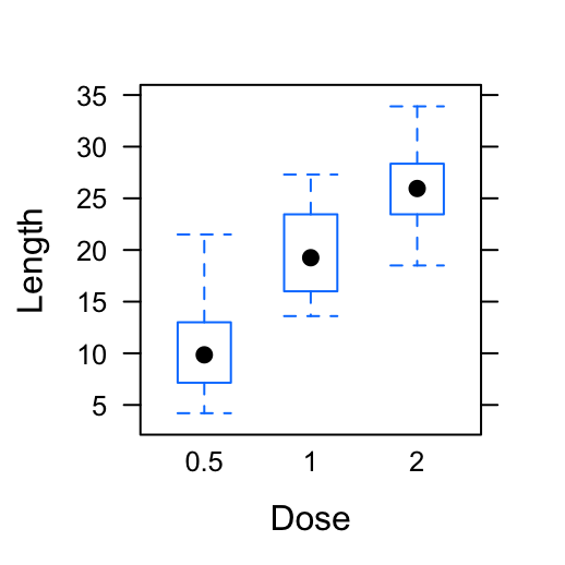
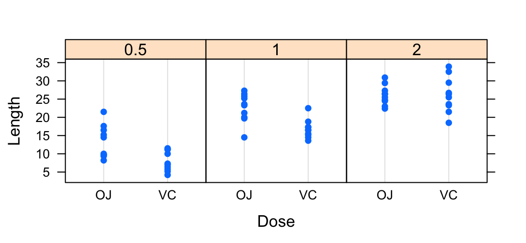
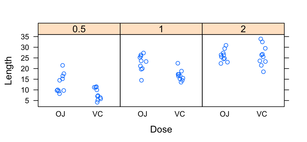
- Plot with multiple groups: Additional argument layout is used: c(3, 1) specifying the number of column and row, respectively
# Box plot
bwplot(len ~ supp | dose, data = ToothGrowth,
layout = c(3, 1),
xlab = "Dose", ylab = "Length")
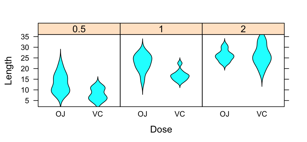
# Violin plot
bwplot(len ~ supp | dose, data = ToothGrowth,
layout = c(3, 1), panel = panel.violin,
xlab = "Dose", ylab = "Length")
# Dot plot
dotplot(len ~ supp | dose, data = ToothGrowth,
layout = c(3, 1),
xlab = "Dose", ylab = "Length")
# Strip plot
stripplot(len ~ supp | dose, data = ToothGrowth,
layout = c(3, 1), jitter.data = TRUE,
xlab = "Dose", ylab = "Length")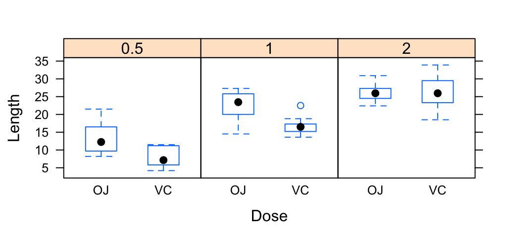
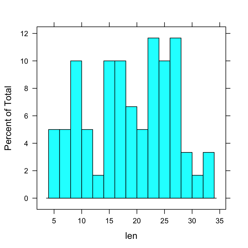
Density plot and Histogram
- Basic plots
densityplot(~ len, data = ToothGrowth,
            plot.points = FALSE)
histogram(~ len, data = ToothGrowth,
            breaks = 20)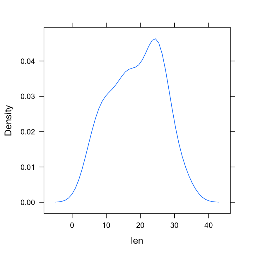
- Plot with multiple groups
densityplot(~ len, groups = dose, data = ToothGrowth,
            plot.points = FALSE, auto.key = TRUE)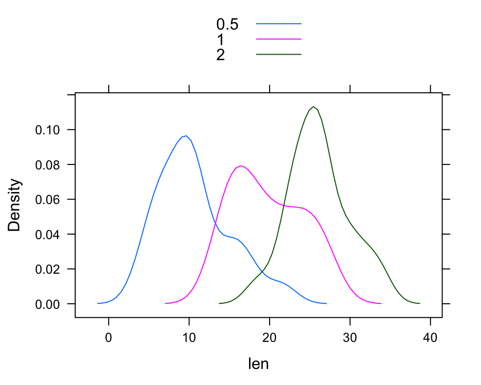
See also
Infos
This analysis has been performed using R statistical software (ver. 3.2.4).
Show me some love with the like buttons below... Thank you and please don't forget to share and comment below!!
Montrez-moi un peu d'amour avec les like ci-dessous ... Merci et n'oubliez pas, s'il vous plaît, de partager et de commenter ci-dessous!
Recommended for You!


Recommended for you
This section contains the best data science and self-development resources to help you on your path.
Books - Data Science
Our Books
- Practical Guide to Cluster Analysis in R by A. Kassambara (Datanovia)
- Practical Guide To Principal Component Methods in R by A. Kassambara (Datanovia)
- Machine Learning Essentials: Practical Guide in R by A. Kassambara (Datanovia)
- R Graphics Essentials for Great Data Visualization by A. Kassambara (Datanovia)
- GGPlot2 Essentials for Great Data Visualization in R by A. Kassambara (Datanovia)
- Network Analysis and Visualization in R by A. Kassambara (Datanovia)
- Practical Statistics in R for Comparing Groups: Numerical Variables by A. Kassambara (Datanovia)
- Inter-Rater Reliability Essentials: Practical Guide in R by A. Kassambara (Datanovia)
Others
- R for Data Science: Import, Tidy, Transform, Visualize, and Model Data by Hadley Wickham & Garrett Grolemund
- Hands-On Machine Learning with Scikit-Learn, Keras, and TensorFlow: Concepts, Tools, and Techniques to Build Intelligent Systems by Aurelien Géron
- Practical Statistics for Data Scientists: 50 Essential Concepts by Peter Bruce & Andrew Bruce
- Hands-On Programming with R: Write Your Own Functions And Simulations by Garrett Grolemund & Hadley Wickham
- An Introduction to Statistical Learning: with Applications in R by Gareth James et al.
- Deep Learning with R by François Chollet & J.J. Allaire
- Deep Learning with Python by François Chollet
Click to follow us on Facebook :
Comment this article by clicking on "Discussion" button (top-right position of this page)