


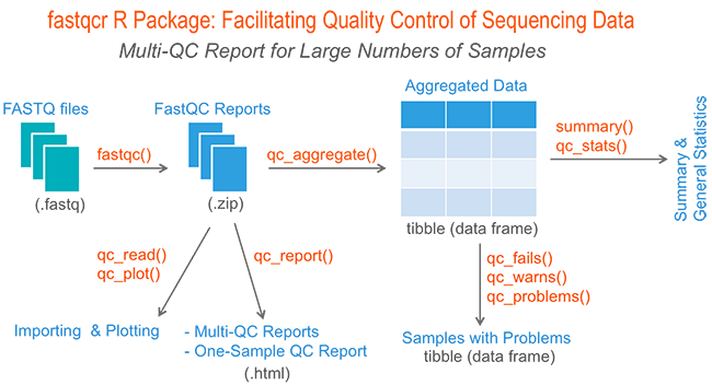
fastqcr: An R Package Facilitating Quality Controls of Sequencing Data for Large Numbers of Samples
Introduction
High throughput sequencing data can contain hundreds of millions of sequences (also known as reads).
The raw sequencing reads may contain PCR primers, adaptors, low quality bases, duplicates and other contaminants coming from the experimental protocols. As these may affect the results of downstream analysis, it’s essential to perform some quality control (QC) checks to ensure that the raw data looks good and there are no problems in your data.
The FastQC tool, written by Simon Andrews at the Babraham Institute, is the most widely used tool to perform quality control for high throughput sequence data. To learn more about the FastQC tool, see this Video Tuorial.
It produces, for each sample, an html report and a ‘zip’ file, which contains a file called fastqc_data.txt and summary.txt.
If you have hundreds of samples, you’re not going to open up each HTML page. You need some way of looking at these data in aggregate.
Therefore, we developed the fastqcr R package, which contains helper functions to easily and automatically parse, aggregate and analyze FastQC reports for large numbers of samples.
Additionally, the fastqcr package provides a convenient solution for building a multi-QC report and a one-sample FastQC report with the result interpretations. The online documentation is available at: https://www.sthda.com/english/rpkgs/fastqcr/.
Examples of QC reports, generated automatically by the fastqcr R package, include:
- Multi-QC report for multiple samples
- One sample QC report (+ interpretation)
- One sample QC report (no interpretation)
In this article, we’ll demonstrate how to perform a quality control of sequencing data. We start by describing how to install and use the FastQC tool. Finally, we’ll describe the fastqcr R package to easily aggregate and analyze FastQC reports for large numbers of samples.
Contents:
- Introduction
- Installation and loading fastqcr
- Quick Start
- Main Functions
- Installing FastQC from R
- Running FastQC from R
- FastQC Reports
- Aggregating Reports
- Summarizing Reports
- Inspecting Problems
- Building an HTML Report
- Importing and Plotting a FastQC QC Report
- Interpreting FastQC Reports
- Useful Links
- Infos
Installation and loading fastqcr
- fastqcr can be installed from CRAN as follow:
install.packages("fastqcr")- Or, install the latest version from GitHub:
if(!require(devtools)) install.packages("devtools")
devtools::install_github("kassambara/fastqcr")- Load fastqcr:
library("fastqcr")Quick Start
library(fastqcr)
# Aggregating Multiple FastQC Reports into a Data Frame
#%%%%%%%%%%%%%%%%%%%%%%%%%%%%%%%%%%%%%%%%%%%%%%%%%%%%%
# Demo QC directory containing zipped FASTQC reports
qc.dir <- system.file("fastqc_results", package = "fastqcr")
qc <- qc_aggregate(qc.dir)
qc
# Inspecting QC Problems
#%%%%%%%%%%%%%%%%%%%%%%%%%%%%%%%%%%%%%%%%%%%%%%%%%%%%%
# See which modules failed in the most samples
qc_fails(qc, "module")
# Or, see which samples failed the most
qc_fails(qc, "sample")
# Building Multi QC Reports
#%%%%%%%%%%%%%%%%%%%%%%%%%%%%%%%%%%%%%%%%%%%%%%%%%%%%%
qc_report(qc.dir, result.file = "multi-qc-report" )
# Building One-Sample QC Reports (+ Interpretation)
#%%%%%%%%%%%%%%%%%%%%%%%%%%%%%%%%%%%%%%%%%%%%%%%%%%%%%
qc.file <- system.file("fastqc_results", "S1_fastqc.zip", package = "fastqcr")
qc_report(qc.file, result.file = "one-sample-report",
          interpret = TRUE)
Main Functions
1) Installing and Running FastQC
fastqc_install(): Install the latest version of FastQC tool on Unix systems (MAC OSX and Linux)
fastqc(): Run the FastQC tool from R.
2) Aggregating and Summarizing Multiple FastQC Reports
qc <- qc_aggregate(): Aggregate multiple FastQC reports into a data frame.
summary(qc): Generates a summary of qc_aggregate.
qc_stats(qc): General statistics of FastQC reports.
3) Inspecting Problems
qc_fails(qc): Displays samples or modules that failed.
qc_warns(qc): Displays samples or modules that warned.
qc_problems(qc): Union of qc_fails() and qc_warns(). Display which samples or modules that failed or warned.
4) Importing and Plotting FastQC Reports
qc_read(): Read FastQC data into R.
qc_plot(qc): Plot FastQC data
5) Building One-Sample and Multi-QC Reports
- qc_report(): Create an HTML file containing FastQC reports of one or multiple files. Inputs can be either a directory containing multiple FastQC reports or a single sample FastQC report.
6) Others
- qc_unzip(): Unzip all zipped files in the qc.dir directory.
Installing FastQC from R
You can install automatically the FastQC tool from R as follow:
fastqc_install()Running FastQC from R
The supported file formats by FastQC include:
- FASTQ
- gzip compressed FASTQ
Suppose that your working directory is organized as follow:
- home
- Documents
- FASTQ
- Documents
where, FASTQ is the directory containing your FASTQ files, for which you want to perform the quality control check.
To run FastQC from R, type this:
fastqc(fq.dir = "~/Documents/FASTQ", # FASTQ files directory
       qc.dir = "~/Documents/FASTQC", # Results direcory
       threads = 4                    # Number of threads
       )
FastQC Reports
For each sample, FastQC performs a series of tests called analysis modules.
These modules include:
- Basic Statistics,
- Per base sequence quality,
- Per tile sequence quality
- Per sequence quality scores,
- Per base sequence content,
- Per sequence GC content,
- Per base N content,
- Sequence Length Distribution,
- Sequence Duplication Levels,
- Overrepresented sequences,
- Adapter Content
- Kmer content
The interpretation of these modules are provided in the official documentation of the FastQC tool.
Aggregating Reports
Here, we provide an R function qc_aggregate() to walk the FastQC result directory, find all the FASTQC zipped output folders, read the fastqc_data.txt and the summary.txt files, and aggregate the information into a data frame.
The fastqc_data.txt file contains the raw data and statistics while the summary.txt file summarizes which tests have been passed.
In the example below, we’ll use a demo FastQC output directory available in the fastqcr package.
library(fastqcr)
# Demo QC dir
qc.dir <- system.file("fastqc_results", package = "fastqcr")
qc.dir
## [1] "/Library/Frameworks/R.framework/Versions/3.3/Resources/library/fastqcr/fastqc_results"# List of files in the directory
list.files(qc.dir)## [1] "S1_fastqc.zip" "S2_fastqc.zip" "S3_fastqc.zip" "S4_fastqc.zip" "S5_fastqc.zip"The demo QC directory contains five zipped folders corresponding to the FastQC output for 5 samples.
Aggregating FastQC reports:
qc <- qc_aggregate(qc.dir)
qc
The aggregated report looks like this:
| sample | module | status | tot.seq | seq.length | pct.gc | pct.dup |
|---|---|---|---|---|---|---|
| S4 | Per tile sequence quality | PASS | 67255341 | 35-76 | 49 | 19.89 |
| S3 | Per base sequence quality | PASS | 67255341 | 35-76 | 49 | 22.14 |
| S3 | Per base N content | PASS | 67255341 | 35-76 | 49 | 22.14 |
| S5 | Per base sequence content | FAIL | 65011962 | 35-76 | 48 | 18.15 |
| S2 | Sequence Duplication Levels | PASS | 50299587 | 35-76 | 48 | 15.70 |
| S1 | Per base sequence content | FAIL | 50299587 | 35-76 | 48 | 17.24 |
| S1 | Overrepresented sequences | PASS | 50299587 | 35-76 | 48 | 17.24 |
| S3 | Basic Statistics | PASS | 67255341 | 35-76 | 49 | 22.14 |
| S1 | Basic Statistics | PASS | 50299587 | 35-76 | 48 | 17.24 |
| S4 | Overrepresented sequences | PASS | 67255341 | 35-76 | 49 | 19.89 |
Column names:
- sample: sample names
- module: fastqc modules
- status: fastqc module status for each sample
- tot.seq: total sequences (i.e.: the number of reads)
- seq.length: sequence length
- pct.gc: percentage of GC content
- pct.dup: percentage of duplicate reads
The table shows, for each sample, the names of tested FastQC modules, the status of the test, as well as, some general statistics including the number of reads, the length of reads, the percentage of GC content and the percentage of duplicate reads.
Once you have the aggregated data you can use the dplyr package to easily inspect modules that failed or warned in samples. For example, the following R code shows samples with warnings and/or failures:
library(dplyr)
qc %>%
  select(sample, module, status) %>%
  filter(status %in% c("WARN", "FAIL")) %>%
arrange(sample)| sample | module | status |
|---|---|---|
| S1 | Per base sequence content | FAIL |
| S1 | Per sequence GC content | WARN |
| S1 | Sequence Length Distribution | WARN |
| S2 | Per base sequence content | FAIL |
| S2 | Per sequence GC content | WARN |
| S2 | Sequence Length Distribution | WARN |
| S3 | Per base sequence content | FAIL |
| S3 | Per sequence GC content | FAIL |
| S3 | Sequence Length Distribution | WARN |
| S4 | Per base sequence content | FAIL |
| S4 | Per sequence GC content | FAIL |
| S4 | Sequence Length Distribution | WARN |
| S5 | Per base sequence content | FAIL |
| S5 | Per sequence GC content | WARN |
| S5 | Sequence Length Distribution | WARN |
In the next section, we’ll describe some easy-to-use functions, available in the fastqcr package, for analyzing the aggregated data.
Summarizing Reports
We start by presenting a summary and general statistics of the aggregated data.
QC Summary
- R function: summary()
- Input data: aggregated data from qc_aggregate()
# Summary of qc
summary(qc)| module | nb_samples | nb_fail | nb_pass | nb_warn | failed | warned |
|---|---|---|---|---|---|---|
| Adapter Content | 5 | 0 | 5 | 0 | NA | NA |
| Basic Statistics | 5 | 0 | 5 | 0 | NA | NA |
| Kmer Content | 5 | 0 | 5 | 0 | NA | NA |
| Overrepresented sequences | 5 | 0 | 5 | 0 | NA | NA |
| Per base N content | 5 | 0 | 5 | 0 | NA | NA |
| Per base sequence content | 5 | 5 | 0 | 0 | S1, S2, S3, S4, S5 | NA |
| Per base sequence quality | 5 | 0 | 5 | 0 | NA | NA |
| Per sequence GC content | 5 | 2 | 0 | 3 | S3, S4 | S1, S2, S5 |
| Per sequence quality scores | 5 | 0 | 5 | 0 | NA | NA |
| Per tile sequence quality | 5 | 0 | 5 | 0 | NA | NA |
| Sequence Duplication Levels | 5 | 0 | 5 | 0 | NA | NA |
| Sequence Length Distribution | 5 | 0 | 0 | 5 | NA | S1, S2, S3, S4, S5 |
Column names:
- module: fastqc modules
- nb_samples: the number of samples tested
- nb_pass, nb_fail, nb_warn: the number of samples that passed, failed and warned, respectively.
- failed, warned: the name of samples that failed and warned, respectively.
The table shows, for each FastQC module, the number and the name of samples that failed or warned.
General statistics
- R function: qc_stats()
- Input data: aggregated data from qc_aggregate()
qc_stats(qc)| sample | pct.dup | pct.gc | tot.seq | seq.length |
|---|---|---|---|---|
| S1 | 17.24 | 48 | 50299587 | 35-76 |
| S2 | 15.70 | 48 | 50299587 | 35-76 |
| S3 | 22.14 | 49 | 67255341 | 35-76 |
| S4 | 19.89 | 49 | 67255341 | 35-76 |
| S5 | 18.15 | 48 | 65011962 | 35-76 |
Column names:
- pct.dup: the percentage of duplicate reads,
- pct.gc: the percentage of GC content,
- tot.seq: total sequences or the number of reads and
- seq.length: sequence length or the length of reads.
The table shows, for each sample, some general statistics such as the total number of reads, the length of reads, the percentage of GC content and the percentage of duplicate reads
Inspecting Problems
Once you’ve got this aggregated data, it’s easy to figure out what (if anything) is wrong with your data.
1) R functions. You can inspect problems per either modules or samples using the following R functions:
- qc_fails(qc): Displays samples or modules that failed.
- qc_warns(qc): Displays samples or modules that warned.
- qc_problems(qc): Union of qc_fails() and qc_warns(). Display which samples or modules that failed or warned.
2) Input data: aggregated data from qc_aggregate()
3) Output data: Returns samples or FastQC modules with failures or warnings. By default, these functions return a compact output format. If you want a stretched format, specify the argument compact = FALSE.
The format and the interpretation of the outputs depend on the additional argument element, which value is one of c(“sample”, “module”).
- If element = “sample” (default), results are samples with failed and/or warned modules. The results contain the following columns:
- sample (sample names),
- nb_problems (the number of modules with problems),
- module (the name of modules with problems).
- If element = “module”, results are modules that failed and/or warned in the most samples. The results contain the following columns:
- module (the name of module with problems),
- nb_problems (the number of samples with problems),
- sample (the name of samples with problems)
Per Module Problems
- Modules that failed in the most samples:
# See which module failed in the most samples
qc_fails(qc, "module")| module | nb_problems | sample |
|---|---|---|
| Per base sequence content | 5 | S1, S2, S3, S4, S5 |
| Per sequence GC content | 2 | S3, S4 |
For each module, the number of problems (failures) and the name of samples, that failed, are shown.
- Modules that warned in the most samples:
# See which module warned in the most samples
qc_warns(qc, "module")| module | nb_problems | sample |
|---|---|---|
| Sequence Length Distribution | 5 | S1, S2, S3, S4, S5 |
| Per sequence GC content | 3 | S1, S2, S5 |
- Modules that failed or warned: Union of qc_fails() and qc_warns()
# See which modules failed or warned.
qc_problems(qc, "module")| module | nb_problems | sample |
|---|---|---|
| Per base sequence content | 5 | S1, S2, S3, S4, S5 |
| Per sequence GC content | 5 | S1, S2, S3, S4, S5 |
| Sequence Length Distribution | 5 | S1, S2, S3, S4, S5 |
The output above is in a compact format. For a stretched format, type this:
qc_problems(qc, "module", compact = FALSE)| module | nb_problems | sample | status |
|---|---|---|---|
| Per base sequence content | 5 | S1 | FAIL |
| Per base sequence content | 5 | S2 | FAIL |
| Per base sequence content | 5 | S3 | FAIL |
| Per base sequence content | 5 | S4 | FAIL |
| Per base sequence content | 5 | S5 | FAIL |
| Per sequence GC content | 5 | S3 | FAIL |
| Per sequence GC content | 5 | S4 | FAIL |
| Per sequence GC content | 5 | S1 | WARN |
| Per sequence GC content | 5 | S2 | WARN |
| Per sequence GC content | 5 | S5 | WARN |
| Sequence Length Distribution | 5 | S1 | WARN |
| Sequence Length Distribution | 5 | S2 | WARN |
| Sequence Length Distribution | 5 | S3 | WARN |
| Sequence Length Distribution | 5 | S4 | WARN |
| Sequence Length Distribution | 5 | S5 | WARN |
In the the stretched format each row correspond to a unique sample. Additionally, the status of each module is specified.
It’s also possible to display problems for one or more specified modules. For example,
qc_problems(qc, "module", name = "Per sequence GC content")| module | nb_problems | sample | status |
|---|---|---|---|
| Per sequence GC content | 5 | S3 | FAIL |
| Per sequence GC content | 5 | S4 | FAIL |
| Per sequence GC content | 5 | S1 | WARN |
| Per sequence GC content | 5 | S2 | WARN |
| Per sequence GC content | 5 | S5 | WARN |
Note that, partial matching of name is allowed. For example, name = “Per sequence GC content” equates to name = “GC content”.
qc_problems(qc, "module", name = "GC content")Per Sample Problems
- Samples with one or more failed modules
# See which samples had one or more failed modules
qc_fails(qc, "sample")| sample | nb_problems | module |
|---|---|---|
| S3 | 2 | Per base sequence content, Per sequence GC content |
| S4 | 2 | Per base sequence content, Per sequence GC content |
| S1 | 1 | Per base sequence content |
| S2 | 1 | Per base sequence content |
| S5 | 1 | Per base sequence content |
For each sample, the number of problems (failures) and the name of modules, that failed, are shown.
- Samples with failed or warned modules:
# See which samples had one or more module with failure or warning
qc_problems(qc, "sample", compact = FALSE)| sample | nb_problems | module | status |
|---|---|---|---|
| S1 | 3 | Per base sequence content | FAIL |
| S1 | 3 | Per sequence GC content | WARN |
| S1 | 3 | Sequence Length Distribution | WARN |
| S2 | 3 | Per base sequence content | FAIL |
| S2 | 3 | Per sequence GC content | WARN |
| S2 | 3 | Sequence Length Distribution | WARN |
| S3 | 3 | Per base sequence content | FAIL |
| S3 | 3 | Per sequence GC content | FAIL |
| S3 | 3 | Sequence Length Distribution | WARN |
| S4 | 3 | Per base sequence content | FAIL |
| S4 | 3 | Per sequence GC content | FAIL |
| S4 | 3 | Sequence Length Distribution | WARN |
| S5 | 3 | Per base sequence content | FAIL |
| S5 | 3 | Per sequence GC content | WARN |
| S5 | 3 | Sequence Length Distribution | WARN |
To specify the name of a sample of interest, type this:
qc_problems(qc, "sample", name = "S1")| sample | nb_problems | module | status |
|---|---|---|---|
| S1 | 3 | Per base sequence content | FAIL |
| S1 | 3 | Per sequence GC content | WARN |
| S1 | 3 | Sequence Length Distribution | WARN |
Building an HTML Report
The function qc_report() can be used to build a report of FastQC outputs. It creates an HTML file containing FastQC reports of one or multiple samples.
Inputs can be either a directory containing multiple FastQC reports or a single sample FastQC report.
Create a Multi-QC Report
We’ll build a multi-qc report for the following demo QC directory:
# Demo QC Directory
qc.dir <- system.file("fastqc_results", package = "fastqcr")
qc.dir
## [1] "/Library/Frameworks/R.framework/Versions/3.3/Resources/library/fastqcr/fastqc_results"# Build a report
qc_report(qc.dir, result.file = "~/Desktop/multi-qc-result",
experiment = "Exome sequencing of colon cancer cell lines")An example of report is available at: fastqcr multi-qc report
Create a One-Sample Report
We’ll build a report for the following demo QC file:
 qc.file <- system.file("fastqc_results", "S1_fastqc.zip", package = "fastqcr")
qc.file
## [1] "/Library/Frameworks/R.framework/Versions/3.3/Resources/library/fastqcr/fastqc_results/S1_fastqc.zip"- One-Sample QC report with plot interpretations:
 qc_report(qc.file, result.file = "one-sample-report-with-interpretation",
   interpret = TRUE)
An example of report is available at: One sample QC report with interpretation
- One-Sample QC report without plot interpretations:
 qc_report(qc.file, result.file = "one-sample-report",
   interpret = FALSE)
An example of report is available at: One sample QC report without interpretation
Importing and Plotting a FastQC QC Report
We’ll visualize the output for sample 1:
# Demo file
qc.file <- system.file("fastqc_results", "S1_fastqc.zip",  package = "fastqcr")
qc.file
## [1] "/Library/Frameworks/R.framework/Versions/3.3/Resources/library/fastqcr/fastqc_results/S1_fastqc.zip"We start by reading the output using the function qc_read(), which returns a list of tibbles containing the data for specified modules:
# Read all modules
qc <- qc_read(qc.file)
# Elements contained in the qc object
names(qc)
## [1] "summary" "basic_statistics" "per_base_sequence_quality" "per_tile_sequence_quality"
## [5] "per_sequence_quality_scores" "per_base_sequence_content" "per_sequence_gc_content" "per_base_n_content"
## [9] "sequence_length_distribution" "sequence_duplication_levels" "overrepresented_sequences" "adapter_content"
## [13] "kmer_content" "total_deduplicated_percentage"The function qc_plot() is used to visualized the data of a specified module. Allowed values for the argument modules include one or the combination of:
- “Summary”,
- “Basic Statistics”,
- “Per base sequence quality”,
- “Per sequence quality scores”,
- “Per base sequence content”,
- “Per sequence GC content”,
- “Per base N content”,
- “Sequence Length Distribution”,
- “Sequence Duplication Levels”,
- “Overrepresented sequences”,
- “Adapter Content”
qc_plot(qc, "Per sequence GC content")
qc_plot(qc, "Per base sequence quality")
qc_plot(qc, "Per sequence quality scores")
qc_plot(qc, "Per base sequence content")
qc_plot(qc, "Sequence duplication levels")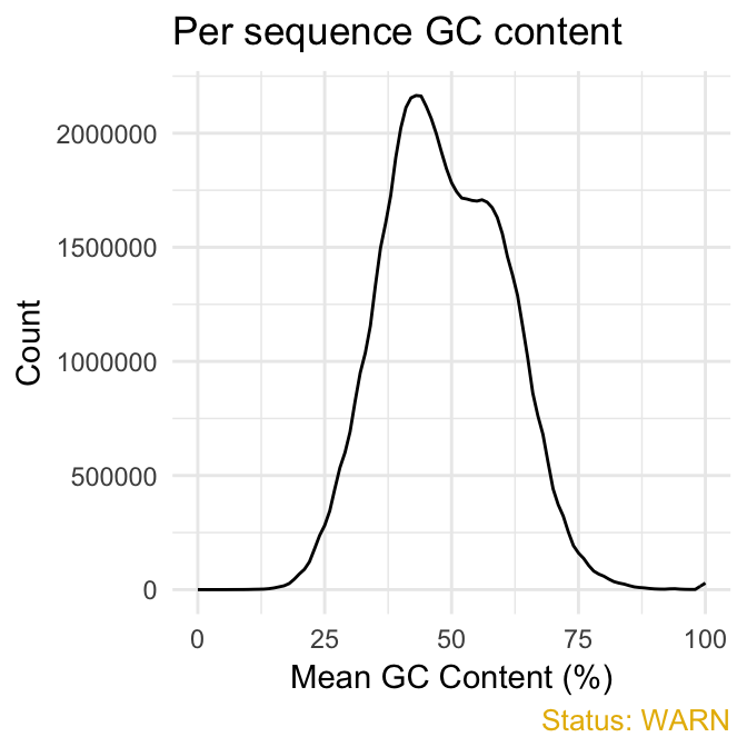
fastqcr
Interpreting FastQC Reports
- Summary shows a summary of the modules which were tested, and the status of the test results:
- normal results (PASS),
- slightly abnormal (WARN: warning)
- or very unusual (FAIL: failure).
Some experiments may be expected to produce libraries which are biased in particular ways. You should treat the summary evaluations therefore as pointers to where you should concentrate your attention and understand why your library may not look normal.
qc_plot(qc, "summary")| status | module | sample |
|---|---|---|
| PASS | Basic Statistics | S1.fastq |
| PASS | Per base sequence quality | S1.fastq |
| PASS | Per tile sequence quality | S1.fastq |
| PASS | Per sequence quality scores | S1.fastq |
| FAIL | Per base sequence content | S1.fastq |
| WARN | Per sequence GC content | S1.fastq |
| PASS | Per base N content | S1.fastq |
| WARN | Sequence Length Distribution | S1.fastq |
| PASS | Sequence Duplication Levels | S1.fastq |
| PASS | Overrepresented sequences | S1.fastq |
| PASS | Adapter Content | S1.fastq |
| PASS | Kmer Content | S1.fastq |
- Basic statistics shows basic data metrics such as:
- Total sequences: the number of reads (total sequences),
- Sequence length: the length of reads (minimum - maximum)
- %GC: GC content
qc_plot(qc, "Basic statistics")| Measure | Value |
|---|---|
| Filename | S1.fastq |
| File type | Conventional base calls |
| Encoding | Sanger / Illumina 1.9 |
| Total Sequences | 50299587 |
| Sequences flagged as poor quality | 0 |
| Sequence length | 35-76 |
| %GC | 48 |
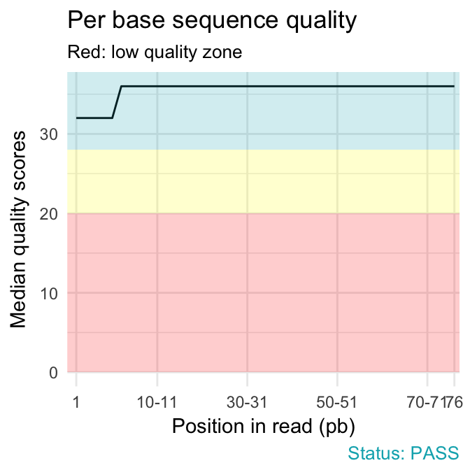
- Per base sequence quality plot depicts the quality scores across all bases at each position in the reads. The background color delimits 3 different zones: very good quality (green), reasonable quality (orange) and poor quality (red). A good sample will have qualities all above 28:
qc_plot(qc, "Per base sequence quality")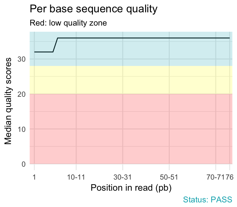
fastqcr
Problems:
- warning if the median for any base is less than 25.
- failure if the median for any base is less than 20.
Common reasons for problems:
-
Degradation of (sequencing chemistry) quality over the duration of long runs. Remedy: Quality trimming.
-
Short loss of quality earlier in the run, which then recovers to produce later good quality sequence. Can be explained by a transient problem with the run (bubbles in the flowcell for example). In these cases trimming is not advisable as it will remove later good sequence, but you might want to consider masking bases during subsequent mapping or assembly.
-
Library with reads of varying length. Warning or error is generated because of very low coverage for a given base range. Before committing to any action, check how many sequences were responsible for triggering an error by looking at the sequence length distribution module results.
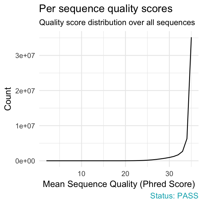
- Per sequence quality scores plot shows the frequencies of quality scores in a sample. It allows you to see if a subset of your sequences have low quality values. If the reads are of good quality, the peak on the plot should be shifted to the right as far as possible (quality > 27).
qc_plot(qc, "Per sequence quality scores")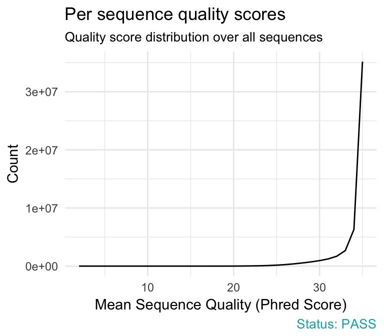
fastqcr
Problems:
- warning if the most frequently observed mean quality is below 27 - this equates to a 0.2% error rate.
- failure if the most frequently observed mean quality is below 20 - this equates to a 1% error rate.
Common reasons for problems:
General loss of quality within a run. Remedy: For long runs this may be alleviated through quality trimming.
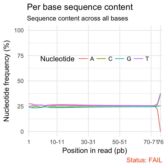
- Per base sequence content shows the four nucleotides’ proportions for each position. In a random library you expect no nucleotide bias and the lines should be almost parallel with each other. In a good sequence composition, the difference between A and T, or G and C is < 10% in any position.
qc_plot(qc, "Per base sequence content")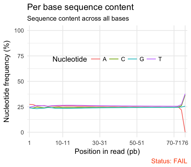
fastqcr
It’s worth noting that some types of library will always produce biased sequence composition, normally at the start of the read. For example, in RNA-Seq data, it is common to have bias at the beginning of the reads. This occurs during RNA-Seq library preparation, when “random” primers are annealed to the start of sequences. These primers are not truly random, and it leads to a variation at the beginning of the reads. We can remove these primers using a trim adaptors tool.
Problems:
- warning if the difference between A and T, or G and C is greater than 10% in any position.
- failure if the difference between A and T, or G and C is greater than 20% in any position.
Common reasons for problems:
-
Overrepresented sequences: adapter dimers or rRNA
-
Biased selection of random primers for RNA-seq. Nearly all RNA-Seq libraries will fail this module because of this bias, but this is not a problem which can be fixed by processing, and it doesn’t seem to adversely affect the ability to measure expression.
-
Biased composition libraries: Some libraries are inherently biased in their sequence composition. For example, library treated with sodium bisulphite, which will then converted most of the cytosines to thymines, meaning that the base composition will be almost devoid of cytosines and will thus trigger an error, despite this being entirely normal for that type of library.
-
Library which has been aggressively adapter trimmed.
- Per sequence GC content plot displays GC distribution over all sequences. In a random library you expect a roughly normal GC content distribution. An unusually sharped or shifted distribution could indicate a contamination or some systematic biases:
qc_plot(qc, "Per sequence GC content")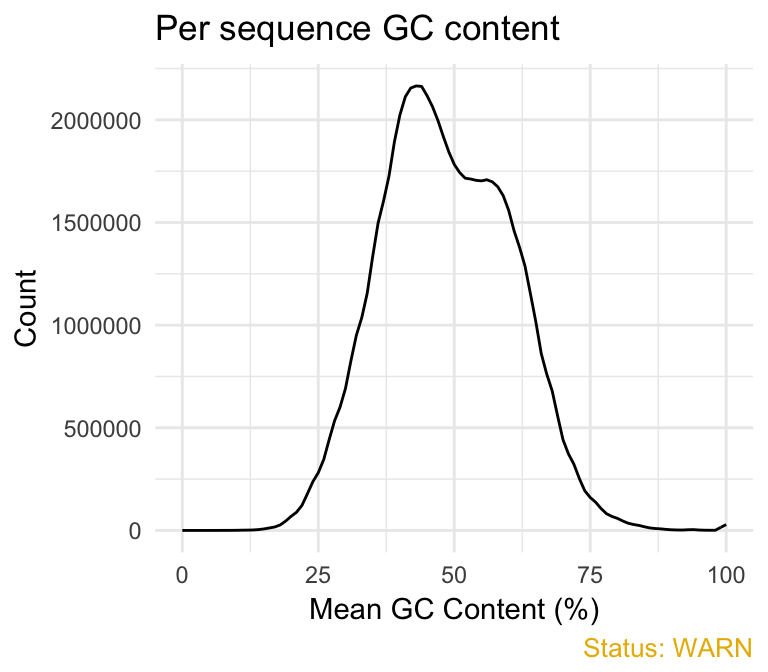
fastqcr
You can generate the theoretical GC content curves files using an R package called fastqcTheoreticalGC written by Mike Love.
- Per base N content. If a sequencer is unable to make a base call with sufficient confidence then it will normally substitute an N rather than a conventional base call. This module plots out the percentage of base calls at each position for which an N was called.
qc_plot(qc, "Per base N content")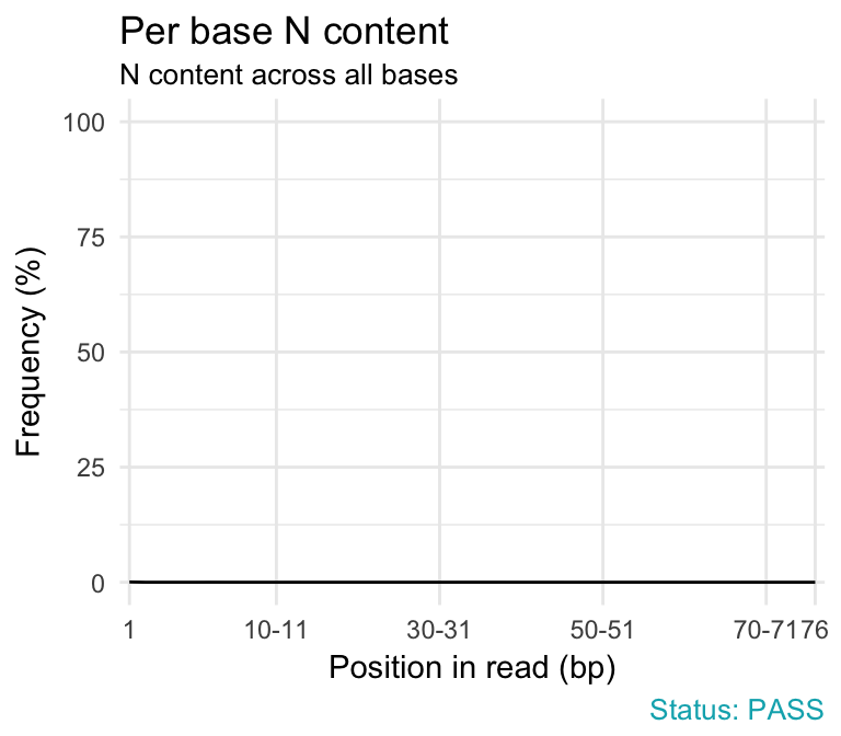
fastqcr
Problems:
- warning if any position shows an N content of >5%.
- failure if any position shows an N content of >20%.
Common reasons for problems:
- General loss of quality.
- Very biased sequence composition in the library.
- Sequence length distribution module reports if all sequences have the same length or not. For some sequencing platforms it is entirely normal to have different read lengths so warnings here can be ignored. In many cases this will produce a simple graph showing a peak only at one size. This module will raise an error if any of the sequences have zero length.
qc_plot(qc, "Sequence length distribution")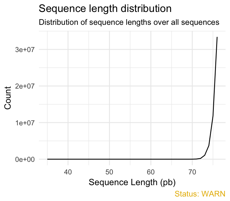
fastqcr
- Sequence duplication levels. This module counts the degree of duplication for every sequence in a library and creates a plot showing the relative number of sequences with different degrees of duplication. A high level of duplication is more likely to indicate some kind of enrichment bias (eg PCR over amplification).
qc_plot(qc, "Sequence duplication levels")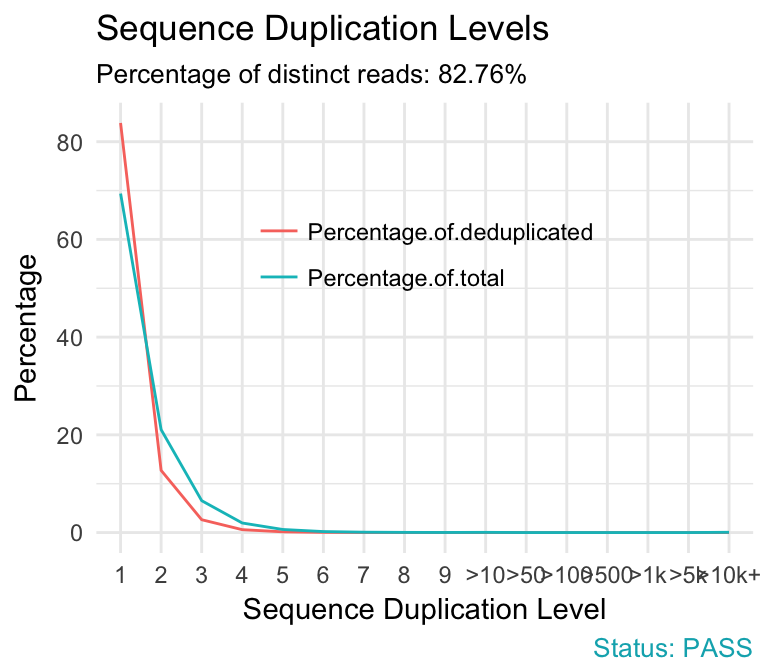
fastqcr
Problems:
- warning if non-unique sequences make up more than 20% of the total.
- failure if non-unique sequences make up more than 50% of the total.
Common reasons for problems:
-
Technical duplicates arising from PCR artifacts
-
Biological duplicates which are natural collisions where different copies of exactly the same sequence are randomly selected.
In RNA-seq data, duplication levels can reach even 40%. Nevertheless, while analyzing transcriptome sequencing data, we should not remove these duplicates because we do not know whether they represent PCR duplicates or high gene expression of our samples.
- Overrepresented sequences section gives information about primer or adaptor contaminations. Finding that a single sequence is very overrepresented in the set either means that it is highly biologically significant, or indicates that the library is contaminated, or not as diverse as you expected. This module lists all of the sequence which make up more than 0.1% of the total.
qc_plot(qc, "Overrepresented sequences")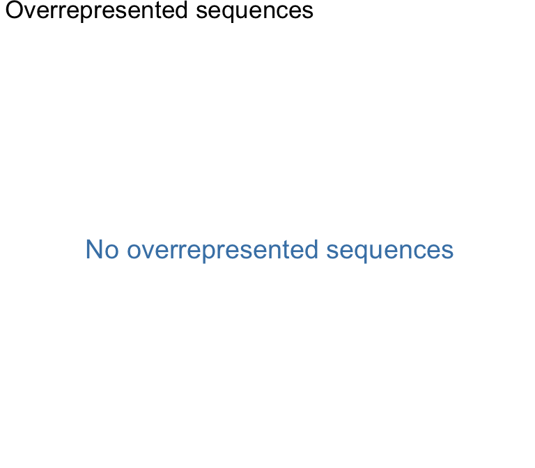
fastqcr
Problems:
- warning if any sequence is found to represent more than 0.1% of the total.
- failure if any sequence is found to represent more than 1% of the total.
Common reasons for problems:
small RNA libraries where sequences are not subjected to random fragmentation, and the same sequence may naturally be present in a significant proportion of the library.
- Adapter content module checks the presence of read-through adapter sequences. It is useful to know if your library contains a significant amount of adapter in order to be able to assess whether you need to adapter trim or not.
qc_plot(qc, "Adapter content")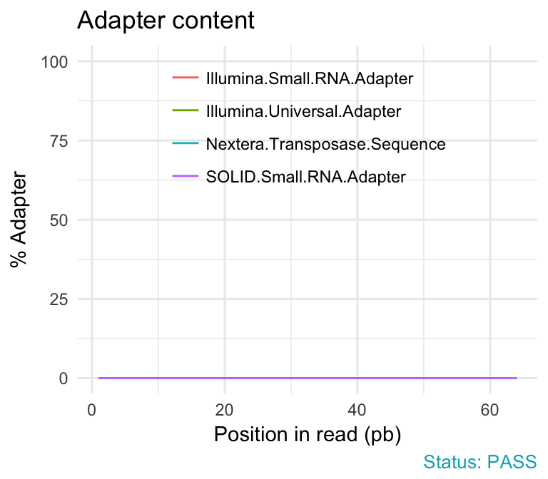
fastqcr
Problems:
- warning if any sequence is present in more than 5% of all reads.
- failure if any sequence is present in more than 10% of all reads.
A warning or failure means that the sequences will need to be adapter trimmed before proceeding with any downstream analysis.
- K-mer content
qc_plot(qc, "Kmer content")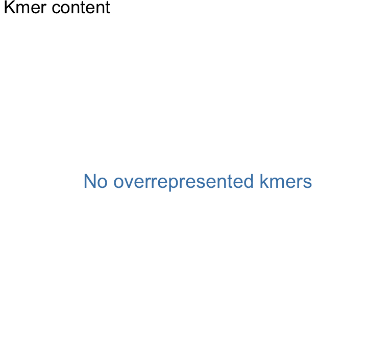
fastqcr
Useful Links
- FastQC report for a good Illumina dataset
- FastQC report for a bad Illumina dataset
- Online documentation for each FastQC report
Infos
This analysis has been performed using R software (ver. 3.3.2).
Show me some love with the like buttons below... Thank you and please don't forget to share and comment below!!
Montrez-moi un peu d'amour avec les like ci-dessous ... Merci et n'oubliez pas, s'il vous plaît, de partager et de commenter ci-dessous!
Recommended for You!


Recommended for you
This section contains the best data science and self-development resources to help you on your path.
Books - Data Science
Our Books
- Practical Guide to Cluster Analysis in R by A. Kassambara (Datanovia)
- Practical Guide To Principal Component Methods in R by A. Kassambara (Datanovia)
- Machine Learning Essentials: Practical Guide in R by A. Kassambara (Datanovia)
- R Graphics Essentials for Great Data Visualization by A. Kassambara (Datanovia)
- GGPlot2 Essentials for Great Data Visualization in R by A. Kassambara (Datanovia)
- Network Analysis and Visualization in R by A. Kassambara (Datanovia)
- Practical Statistics in R for Comparing Groups: Numerical Variables by A. Kassambara (Datanovia)
- Inter-Rater Reliability Essentials: Practical Guide in R by A. Kassambara (Datanovia)
Others
- R for Data Science: Import, Tidy, Transform, Visualize, and Model Data by Hadley Wickham & Garrett Grolemund
- Hands-On Machine Learning with Scikit-Learn, Keras, and TensorFlow: Concepts, Tools, and Techniques to Build Intelligent Systems by Aurelien Géron
- Practical Statistics for Data Scientists: 50 Essential Concepts by Peter Bruce & Andrew Bruce
- Hands-On Programming with R: Write Your Own Functions And Simulations by Garrett Grolemund & Hadley Wickham
- An Introduction to Statistical Learning: with Applications in R by Gareth James et al.
- Deep Learning with R by François Chollet & J.J. Allaire
- Deep Learning with Python by François Chollet
Click to follow us on Facebook :
Comment this article by clicking on "Discussion" button (top-right position of this page)