


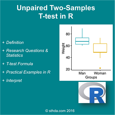
Unpaired Two-Samples T-test in R
- What is unpaired two-samples t-test?
- Research questions and statistical hypotheses
- Formula of unpaired two-samples t-test
- Visualize your data and compute unpaired two-samples t-test in R
- Install ggpubr R package for data visualization
- R function to compute unpaired two-samples t-test
- Import your data into R
- Check your data
- Visualize your data using box plots
- Preleminary test to check independent t-test assumptions
- Compute unpaired two-samples t-test
- Interpretation of the result
- Access to the values returned by t.test() function
- Online unpaired two-samples t-test calculator
- See also
- Infos
What is unpaired two-samples t-test?
For example, suppose that we have measured the weight of 100 individuals: 50 women (group A) and 50 men (group B). We want to know if the mean weight of women (\(m_A\)) is significantly different from that of men (\(m_B\)).
In this case, we have two unrelated (i.e., independent or unpaired) groups of samples. Therefore, it’s possible to use an independent t-test to evaluate whether the means are different.
Note that, unpaired two-samples t-test can be used only under certain conditions:
- when the two groups of samples (A and B), being compared, are normally distributed. This can be checked using Shapiro-Wilk test.
- and when the variances of the two groups are equal. This can be checked using F-test.
This article describes the formula of the independent t-test and provides pratical examples in R.
Research questions and statistical hypotheses
Typical research questions are:
- whether the mean of group A (\(m_A\)) is equal to the mean of group B (\(m_B\))?
- whether the mean of group A (\(m_A\)) is less than the mean of group B (\(m_B\))?
- whether the mean of group A (\(m_A\)) is greather than the mean of group B (\(m_B\))?
In statistics, we can define the corresponding null hypothesis (\(H_0\)) as follow:
- \(H_0: m_A = m_B\)
- \(H_0: m_A \leq m_B\)
- \(H_0: m_A \geq m_B\)
The corresponding alternative hypotheses (\(H_a\)) are as follow:
- \(H_a: m_A \ne m_B\) (different)
- \(H_a: m_A > m_B\) (greater)
- \(H_a: m_A < m_B\) (less)
Note that:
- Hypotheses 1) are called two-tailed tests
- Hypotheses 2) and 3) are called one-tailed tests
Formula of unpaired two-samples t-test
- Classical t-test:
If the variance of the two groups are equivalent (homoscedasticity), the t-test value, comparing the two samples (\(A\) and \(B\)), can be calculated as follow.
\[ t = \frac{m_A - m_B}{\sqrt{ \frac{S^2}{n_A} + \frac{S^2}{n_B} }} \]
where,
- \(m_A\) and \(m_B\) represent the mean value of the group A and B, respectively.
- \(n_A\) and \(n_B\) represent the sizes of the group A and B, respectively.
- \(S^2\) is an estimator of the pooled variance of the two groups. It can be calculated as follow :
\[ S^2 = \frac{\sum{(x-m_A)^2}+\sum{(x-m_B)^2}}{n_A+n_B-2} \]
with degrees of freedom (df): \(df = n_A + n_B - 2\).
2.Welch t-statistic:
If the variances of the two groups being compared are different (heteroscedasticity), it’s possible to use the Welch t test, an adaptation of Student t-test.
Welch t-statistic is calculated as follow :
\[ t = \frac{m_A - m_B}{\sqrt{ \frac{S_A^2}{n_A} + \frac{S_B^2}{n_B} }} \]
where, \(S_A\) and \(S_B\) are the standard deviation of the the two groups A and B, respectively.
Unlike the classic Student’s t-test, Welch t-test formula involves the variance of each of the two groups (\(S_A^2\) and \(S_B^2\)) being compared. In other words, it does not use the pooled variance\(S\).
The degrees of freedom of Welch t-test is estimated as follow :
\[ df = (\frac{S_A^2}{n_A}+ \frac{S_B^2}{n_B^2}) / (\frac{S_A^4}{n_A^2(n_B-1)} + \frac{S_B^4}{n_B^2(n_B-1)} ) \]
A p-value can be computed for the corresponding absolute value of t-statistic (|t|).
Note that, the Welch t-test is considered as the safer one. Usually, the results of the classical t-test and the Welch t-test are very similar unless both the group sizes and the standard deviations are very different.
How to interpret the results?
If the p-value is inferior or equal to the significance level 0.05, we can reject the null hypothesis and accept the alternative hypothesis. In other words, we can conclude that the mean values of group A and B are significantly different.
Visualize your data and compute unpaired two-samples t-test in R
Install ggpubr R package for data visualization
You can draw R base graphs as described at this link: R base graphs. Here, we’ll use the ggpubr R package for an easy ggplot2-based data visualization
- Install the latest version from GitHub as follow (recommended):
# Install
if(!require(devtools)) install.packages("devtools")
devtools::install_github("kassambara/ggpubr")- Or, install from CRAN as follow:
install.packages("ggpubr")R function to compute unpaired two-samples t-test
To perform two-samples t-test comparing the means of two independent samples (x & y), the R function t.test() can be used as follow:
t.test(x, y, alternative = "two.sided", var.equal = FALSE)- x,y: numeric vectors
- alternative: the alternative hypothesis. Allowed value is one of “two.sided” (default), “greater” or “less”.
- var.equal: a logical variable indicating whether to treat the two variances as being equal. If TRUE then the pooled variance is used to estimate the variance otherwise the Welch test is used.
Import your data into R
Prepare your data as specified here: Best practices for preparing your data set for R
Save your data in an external .txt tab or .csv files
Import your data into R as follow:
# If .txt tab file, use this
my_data <- read.delim(file.choose())
# Or, if .csv file, use this
my_data <- read.csv(file.choose())
Here, we’ll use an example data set, which contains the weight of 18 individuals (9 women and 9 men):
# Data in two numeric vectors
women_weight <- c(38.9, 61.2, 73.3, 21.8, 63.4, 64.6, 48.4, 48.8, 48.5)
men_weight <- c(67.8, 60, 63.4, 76, 89.4, 73.3, 67.3, 61.3, 62.4)
# Create a data frame
my_data <- data.frame(
                group = rep(c("Woman", "Man"), each = 9),
                weight = c(women_weight,  men_weight)
                )
We want to know, if the average women’s weight differs from the average men’s weight?
Check your data
# Print all data
print(my_data)
group weight
1 Woman 38.9
2 Woman 61.2
3 Woman 73.3
4 Woman 21.8
5 Woman 63.4
6 Woman 64.6
7 Woman 48.4
8 Woman 48.8
9 Woman 48.5
10 Man 67.8
11 Man 60.0
12 Man 63.4
13 Man 76.0
14 Man 89.4
15 Man 73.3
16 Man 67.3
17 Man 61.3
18 Man 62.4It’s possible to compute summary statistics (mean and sd) by groups. The dplyr package can be used.
- To install dplyr package, type this:
install.packages("dplyr")- Compute summary statistics by groups:
library(dplyr)
group_by(my_data, group) %>%
  summarise(
    count = n(),
    mean = mean(weight, na.rm = TRUE),
    sd = sd(weight, na.rm = TRUE)
  )
Source: local data frame [2 x 4]
group count mean sd
(fctr) (int) (dbl) (dbl)
1 Man 9 68.98889 9.375426
2 Woman 9 52.10000 15.596714Visualize your data using box plots
# Plot weight by group and color by group
library("ggpubr")
ggboxplot(my_data, x = "group", y = "weight",
          color = "group", palette = c("#00AFBB", "#E7B800"),
        ylab = "Weight", xlab = "Groups")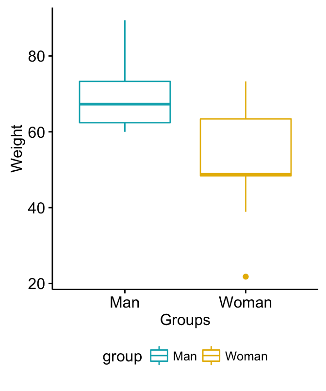
Unpaired Two-Samples Student’s T-test in R
Preleminary test to check independent t-test assumptions
Assumption 1: Are the two samples independents?
Yes, since the samples from men and women are not related.
Assumtion 2: Are the data from each of the 2 groups follow a normal distribution?
Use Shapiro-Wilk normality test as described at: Normality Test in R. - Null hypothesis: the data are normally distributed - Alternative hypothesis: the data are not normally distributed
We’ll use the functions with() and shapiro.test() to compute Shapiro-Wilk test for each group of samples.
# Shapiro-Wilk normality test for Men's weights
with(my_data, shapiro.test(weight[group == "Man"]))# p = 0.1
# Shapiro-Wilk normality test for Women's weights
with(my_data, shapiro.test(weight[group == "Woman"])) # p = 0.6
From the output, the two p-values are greater than the significance level 0.05 implying that the distribution of the data are not significantly different from the normal distribution. In other words, we can assume the normality.
Note that, if the data are not normally distributed, it’s recommended to use the non parametric two-samples Wilcoxon rank test.
Assumption 3. Do the two populations have the same variances?
We’ll use F-test to test for homogeneity in variances. This can be performed with the function var.test() as follow:
res.ftest <- var.test(weight ~ group, data = my_data)
res.ftest
    F test to compare two variances
data:  weight by group
F = 0.36134, num df = 8, denom df = 8, p-value = 0.1714
alternative hypothesis: true ratio of variances is not equal to 1
95 percent confidence interval:
 0.08150656 1.60191315
sample estimates:
ratio of variances
0.3613398 Compute unpaired two-samples t-test
Question : Is there any significant difference between women and men weights?
1) Compute independent t-test - Method 1: The data are saved in two different numeric vectors.
# Compute t-test
res <- t.test(women_weight, men_weight, var.equal = TRUE)
res
    Two Sample t-test
data:  women_weight and men_weight
t = -2.7842, df = 16, p-value = 0.01327
alternative hypothesis: true difference in means is not equal to 0
95 percent confidence interval:
 -29.748019  -4.029759
sample estimates:
mean of x mean of y
 52.10000  68.98889
2) Compute independent t-test - Method 2: The data are saved in a data frame.
# Compute t-test
res <- t.test(weight ~ group, data = my_data, var.equal = TRUE)
res
    Two Sample t-test
data:  weight by group
t = 2.7842, df = 16, p-value = 0.01327
alternative hypothesis: true difference in means is not equal to 0
95 percent confidence interval:
  4.029759 29.748019
sample estimates:
  mean in group Man mean in group Woman
           68.98889            52.10000
As you can see, the two methods give the same results.
In the result above :
- t is the t-test statistic value (t = 2.784),
- df is the degrees of freedom (df= 16),
- p-value is the significance level of the t-test (p-value = 0.01327).
- conf.int is the confidence interval of the mean at 95% (conf.int = [4.0298, 29.748]);
- sample estimates is he mean value of the sample (mean = 68.9888889, 52.1).
Note that:
- if you want to test whether the average men’s weight is less than the average women’s weight, type this:
t.test(weight ~ group, data = my_data,
var.equal = TRUE, alternative = "less")- Or, if you want to test whether the average men’s weight is greater than the average women’s weight, type this
t.test(weight ~ group, data = my_data,
        var.equal = TRUE, alternative = "greater")
Interpretation of the result
The p-value of the test is 0.01327, which is less than the significance level alpha = 0.05. We can conclude that men’s average weight is significantly different from women’s average weight with a p-value = 0.01327.
Access to the values returned by t.test() function
The result of t.test() function is a list containing the following components:
- statistic: the value of the t test statistics
- parameter: the degrees of freedom for the t test statistics
- p.value: the p-value for the test
- conf.int: a confidence interval for the mean appropriate to the specified alternative hypothesis.
- estimate: the means of the two groups being compared (in the case of independent t test) or difference in means (in the case of paired t test).
The format of the R code to use for getting these values is as follow:
# printing the p-value
res$p.value
[1] 0.0132656# printing the mean
res$estimate mean in group Man mean in group Woman
68.98889 52.10000 # printing the confidence interval
res$conf.int[1] 4.029759 29.748019
attr(,"conf.level")
[1] 0.95Online unpaired two-samples t-test calculator
You can perform unpaired two-samples t-test, online, without any installation by clicking the following link:
See also
- Compare one-sample mean to a standard known mean
- Compare the means of two independent groups
Infos
This analysis has been performed using R software (ver. 3.2.4).
Show me some love with the like buttons below... Thank you and please don't forget to share and comment below!!
Montrez-moi un peu d'amour avec les like ci-dessous ... Merci et n'oubliez pas, s'il vous plaît, de partager et de commenter ci-dessous!
Recommended for You!


Recommended for you
This section contains the best data science and self-development resources to help you on your path.
Books - Data Science
Our Books
- Practical Guide to Cluster Analysis in R by A. Kassambara (Datanovia)
- Practical Guide To Principal Component Methods in R by A. Kassambara (Datanovia)
- Machine Learning Essentials: Practical Guide in R by A. Kassambara (Datanovia)
- R Graphics Essentials for Great Data Visualization by A. Kassambara (Datanovia)
- GGPlot2 Essentials for Great Data Visualization in R by A. Kassambara (Datanovia)
- Network Analysis and Visualization in R by A. Kassambara (Datanovia)
- Practical Statistics in R for Comparing Groups: Numerical Variables by A. Kassambara (Datanovia)
- Inter-Rater Reliability Essentials: Practical Guide in R by A. Kassambara (Datanovia)
Others
- R for Data Science: Import, Tidy, Transform, Visualize, and Model Data by Hadley Wickham & Garrett Grolemund
- Hands-On Machine Learning with Scikit-Learn, Keras, and TensorFlow: Concepts, Tools, and Techniques to Build Intelligent Systems by Aurelien Géron
- Practical Statistics for Data Scientists: 50 Essential Concepts by Peter Bruce & Andrew Bruce
- Hands-On Programming with R: Write Your Own Functions And Simulations by Garrett Grolemund & Hadley Wickham
- An Introduction to Statistical Learning: with Applications in R by Gareth James et al.
- Deep Learning with R by François Chollet & J.J. Allaire
- Deep Learning with Python by François Chollet
Click to follow us on Facebook :
Comment this article by clicking on "Discussion" button (top-right position of this page)