


CA in R Using FactoMineR: Quick Scripts and Videos
This page shows quick start R code to compute correspondence analysis- CA in R using the FactoMineR package.
Additionaly, we present series of course videos on correspondence analysis, which is a multivariate analysis tool for analyzing large contingency tables formed by two categorical variables. The aim isto study the association between row and column elements.
In the videos, the instructors start by explaining the theory and the key concept behind CA. Next, they provide provide practical examples and interpretation of CA in R programming language.
Contents:
Quick start R code
- Install FactoMineR package:
install.packages("FactoMineR")- Compute CA using the demo data set children [in FactoMineR]. The data set is a contingency table that summarizes the answers given by different categories of people to the following question : according to you, what are the reasons that can make hesitate a woman or a couple to have children?
library(FactoMineR)
data("children")
res.ca <- CA(children,
             row.sup = 15:18,  # Supplementary rows
             col.sup = 6:8,    # Supplementary columns
             graph = FALSE)
Key terms:
- Active rows and columns are used during the correspondence analysis.
- Supplementary rows and columns: their coordinates will be predicted after the CA.
- Visualize eigenvalues (scree plot). Show the percentage of variances explained by each principal component.
eig.val <- res.ca$eig
barplot(eig.val[, 2],
        names.arg = 1:nrow(eig.val),
        main = "Variances Explained by Dimensions (%)",
        xlab = "Principal Dimensions",
        ylab = "Percentage of variances",
        col ="steelblue")
# Add connected line segments to the plot
lines(x = 1:nrow(eig.val), eig.val[, 2],
      type = "b", pch = 19, col = "red")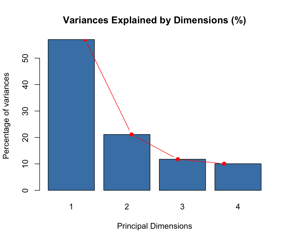
- Biplot of row and column variables showing the association between row and column elements.
plot(res.ca, autoLab = "yes")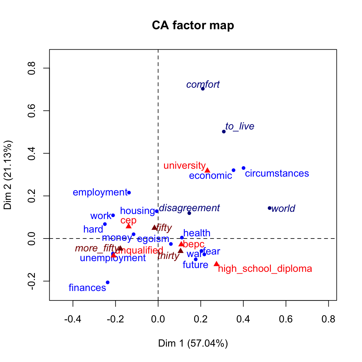
blue: row pointsdarkblue: supplementary rowsred: column pointsdarkred: supplementary columns
To plot only the row variables, specify the argumenet invisible = “col”. For column variables, type invisible = “row”.
For ggplot2-based visualization, read this: CA - Correspondence Analysis in R: Essentials
- Access to the results:
# Eigenvalues
res.ca$eig
# Results for row variables
res.row <- res.ca$row
res.row$coord          # Coordinates
res.row$contrib        # Contributions to the PCs
res.row$cos2           # Quality of representation
# Results for column variables
res.col <- res.ca$col
res.col$coord          # Coordinates
res.col$contrib        # Contributions to the PCs
res.col$cos2           # Quality of representation
Theory and key concepts
Introduction and data types
This video describes the data and key notations, as well as, the questions that can be investigated by correspondence analysis. You’ll we see that the main point of correspondence analysis is studying the links between pairs of qualitative variables.
Visualizing the row and column clouds
This video presents how to plot row and column points on the same graph.
Inertia
This video presents the importance of inertia in the interpretation of correspondence analysis.
Simultaneous representation
This video describes how to plot simultaneously row and column elements on the same plot.
Interpretation
This video introduces the concept of quality of representation and contribution.
Course video materials
Correspondence analysis examples in R
CA in practice with FactoMineR
Text mining with correspondence analysis
Graphical user interface: Factoshiny
The package Factoshiny provides user graphical interface for correspondence analysis.
Automatic interpretation: FactoInvestigate
The package FactoInvestigate can be used to generate automatically a report for correspondence analysis.
Learn more in our previous article: FactoInvestigate R Package: Automatic Reports and Interpretation of Principal Component Analyses


