Usage

The format of rquery.wordcloud() function is shown below :

rquery.wordcloud(x, type=c("text", "url", "file"), 
        lang="english", excludeWords = NULL, 
        textStemming = FALSE,  colorPalette="Dark2",
        max.words=200)

Required R packages

The following packages are required for the rquery.wordcloud() function :

• tm for text mining
• SnowballC for text stemming
• wordcloud for generating word cloud images
• RCurl and XML packages to download and parse web pages
• RColorBrewer for color palettes

Install these packages, before using the function rquery.wordcloud, as follow :

install.packages(c("tm", "SnowballC", "wordcloud", "RColorBrewer", "RCurl", "XML")

Create a word cloud from a plain text file

Plain text file can be easily created using your favorite text editor (e.g : Word). “I have a dream speech” (from Martin Luther King) is processed in the following example but you can use any text you want :

• Copy and paste your text in a plain text file
• Save the file (e.g : ml.txt)

Generate the word cloud using the R code below :

source('http://www.sthda.com/upload/rquery_wordcloud.r')
filePath <- "http://www.sthda.com/sthda/RDoc/example-files/martin-luther-king-i-have-a-dream-speech.txt"
res<-rquery.wordcloud(filePath, type ="file", lang = "english")

Change the arguments max.words and min.freq to plot more words :

• max.words : maximum number of words to be plotted.
• min.freq : words with frequency below min.freq will not be plotted

res<-rquery.wordcloud(filePath, type ="file", lang = "english",
                 min.freq = 1,  max.words = 200)

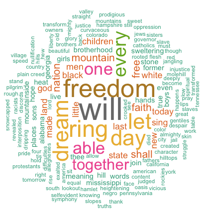
The above image clearly shows that “Will”, “freedom”, “dream”, “day” and “together” are the five most frequent words in Martin Luther King “I have a dream speech”.

Change the color of the word cloud

The color of the word cloud can be changed using the argument colorPalette.

Allowed values for colorPalete :

• a color name (e.g.: colorPalette = “blue”)
• a color code (e.g.: colorPalette = “#FF1425”)
• a name of a color palette taken from RColorBrewer package (e.g.: colorPalette = “Dark2”)

The color palettes associated to RColorBrewer package are shown below :

Color palette can be changed as follow :

# Reds color palette
res<-rquery.wordcloud(filePath, type ="file", lang = "english",
                      colorPalette = "Reds")
# RdBu color palette
res<-rquery.wordcloud(filePath, type ="file", lang = "english",
                      colorPalette = "RdBu")
# use unique color
res<-rquery.wordcloud(filePath, type ="file", lang = "english",
                      colorPalette = "black")

Operations on the result of rquery.wordcloud() function

As mentioned above, the result of rquery.wordcloud() is a list containing two objects :

• tdm : term-document matrix
• freqTable : frequency table

tdm <- res$tdm
freqTable <- res$freqTable

# Show the top10 words and their frequency
head(freqTable, 10)

             word freq
will         will   17
freedom   freedom   13
ring         ring   12
day           day   11
dream       dream   11
let           let   11
every       every    9
able         able    8
one           one    8
together together    7

# Bar plot of the frequency for the top10
barplot(freqTable[1:10,]$freq, las = 2, 
        names.arg = freqTable[1:10,]$word,
        col ="lightblue", main ="Most frequent words",
        ylab = "Word frequencies")

findFreqTerms(tdm, lowfreq = 4)

 [1] "able"     "day"      "dream"    "every"    "faith"    "free"     "freedom"  "let"      "mountain" "nation"  
[11] "one"      "ring"     "shall"    "together" "will"    

findAssocs(tdm, terms = "freedom", corlimit = 0.3)

             freedom
let             0.89
ring            0.86
mississippi     0.34
mountainside    0.34
stone           0.34
every           0.32
mountain        0.32
state           0.32

Create a word cloud of a web page

In this section we’ll make a tag cloud of the following web page :

http://www.sthda.com/english/wiki/create-and-format-powerpoint-documents-from-r-software

url = "http://www.sthda.com/english/wiki/create-and-format-powerpoint-documents-from-r-software"
rquery.wordcloud(x=url, type="url")

The above word cloud shows that “powerpoint”, “doc”, “slide”, “reporters” are among the most important words on the analyzed web page. This confirms the fact that the article is about creating PowerPoint document using ReporteRs package in R

R code of rquery.wordcloud function

#++++++++++++++++++++++++++++++++++
# rquery.wordcloud() : Word cloud generator
# - http://www.sthda.com
#+++++++++++++++++++++++++++++++++++
# x : character string (plain text, web url, txt file path)
# type : specify whether x is a plain text, a web page url or a file path
# lang : the language of the text
# excludeWords : a vector of words to exclude from the text
# textStemming : reduces words to their root form
# colorPalette : the name of color palette taken from RColorBrewer package, 
  # or a color name, or a color code
# min.freq : words with frequency below min.freq will not be plotted
# max.words : Maximum number of words to be plotted. least frequent terms dropped
# value returned by the function : a list(tdm, freqTable)
rquery.wordcloud <- function(x, type=c("text", "url", "file"), 
                          lang="english", excludeWords=NULL, 
                          textStemming=FALSE,  colorPalette="Dark2",
                          min.freq=3, max.words=200)
{ 
  library("tm")
  library("SnowballC")
  library("wordcloud")
  library("RColorBrewer") 
  
  if(type[1]=="file") text <- readLines(x)
  else if(type[1]=="url") text <- html_to_text(x)
  else if(type[1]=="text") text <- x
  
  # Load the text as a corpus
  docs <- Corpus(VectorSource(text))
  # Convert the text to lower case
  docs <- tm_map(docs, content_transformer(tolower))
  # Remove numbers
  docs <- tm_map(docs, removeNumbers)
  # Remove stopwords for the language 
  docs <- tm_map(docs, removeWords, stopwords(lang))
  # Remove punctuations
  docs <- tm_map(docs, removePunctuation)
  # Eliminate extra white spaces
  docs <- tm_map(docs, stripWhitespace)
  # Remove your own stopwords
  if(!is.null(excludeWords)) 
    docs <- tm_map(docs, removeWords, excludeWords) 
  # Text stemming
  if(textStemming) docs <- tm_map(docs, stemDocument)
  # Create term-document matrix
  tdm <- TermDocumentMatrix(docs)
  m <- as.matrix(tdm)
  v <- sort(rowSums(m),decreasing=TRUE)
  d <- data.frame(word = names(v),freq=v)
  # check the color palette name 
  if(!colorPalette %in% rownames(brewer.pal.info)) colors = colorPalette
  else colors = brewer.pal(8, colorPalette) 
  # Plot the word cloud
  set.seed(1234)
  wordcloud(d$word,d$freq, min.freq=min.freq, max.words=max.words,
            random.order=FALSE, rot.per=0.35, 
            use.r.layout=FALSE, colors=colors)
  
  invisible(list(tdm=tdm, freqTable = d))
}
#++++++++++++++++++++++
# Helper function
#++++++++++++++++++++++
# Download and parse webpage
html_to_text<-function(url){
  library(RCurl)
  library(XML)
  # download html
  html.doc <- getURL(url)  
  #convert to plain text
  doc = htmlParse(html.doc, asText=TRUE)
 # "//text()" returns all text outside of HTML tags.
 # We also don’t want text such as style and script codes
  text <- xpathSApply(doc, "//text()[not(ancestor::script)][not(ancestor::style)][not(ancestor::noscript)][not(ancestor::form)]", xmlValue)
  # Format text vector into one character string
  return(paste(text, collapse = " "))
}