


Text mining and word cloud fundamentals in R : 5 simple steps you should know
Text mining methods allow us to highlight the most frequently used keywords in a paragraph of texts. One can create a word cloud, also referred as text cloud or tag cloud, which is a visual representation of text data.
The procedure of creating word clouds is very simple in R if you know the different steps to execute. The text mining package (tm) and the word cloud generator package (wordcloud) are available in R for helping us to analyze texts and to quickly visualize the keywords as a word cloud.
In this article, we’ll describe, step by step, how to generate word clouds using the R software.
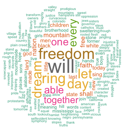
word cloud and text mining, I have a dream speech from Martin luther king
3 reasons you should use word clouds to present your text data
- Word clouds add simplicity and clarity. The most used keywords stand out better in a word cloud
- Word clouds are a potent communication tool. They are easy to understand, to be shared and are impactful
- Word clouds are visually engaging than a table data
Who is using word clouds ?
- Researchers : for reporting qualitative data
- Marketers : for highlighting the needs and pain points of customers
- Educators : to support essential issues
- Politicians and journalists
- social media sites : to collect, analyze and share user sentiments
The 5 main steps to create word clouds in R
Step 1: Create a text file
In the following examples, I’ll process the “I have a dream speech” from “Martin Luther King” but you can use any text you want :
- Copy and paste the text in a plain text file (e.g : ml.txt)
- Save the file
Note that, the text should be saved in a plain text (.txt) file format using your favorite text editor.
Step 2 : Install and load the required packages
Type the R code below, to install and load the required packages:
# Install
install.packages("tm")  # for text mining
install.packages("SnowballC") # for text stemming
install.packages("wordcloud") # word-cloud generator
install.packages("RColorBrewer") # color palettes
# Load
library("tm")
library("SnowballC")
library("wordcloud")
library("RColorBrewer")
Step 3 : Text mining
load the text
The text is loaded using Corpus() function from text mining (tm) package. Corpus is a list of a document (in our case, we only have one document).
- We start by importing the text file created in Step 1
To import the file saved locally in your computer, type the following R code. You will be asked to choose the text file interactively.
text <- readLines(file.choose())In the example below, I’ll load a .txt file hosted on STHDA website:
# Read the text file from internet
filePath <- "https://www.sthda.com/sthda/RDoc/example-files/martin-luther-king-i-have-a-dream-speech.txt"
text <- readLines(filePath)- Load the data as a corpus
# Load the data as a corpus
docs <- Corpus(VectorSource(text))
VectorSource() function creates a corpus of character vectors
- Inspect the content of the document
inspect(docs)Text transformation
Transformation is performed using tm_map() function to replace, for example, special characters from the text.
Replacing “/”, “@” and “|” with space:
toSpace <- content_transformer(function (x , pattern ) gsub(pattern, " ", x))
docs <- tm_map(docs, toSpace, "/")
docs <- tm_map(docs, toSpace, "@")
docs <- tm_map(docs, toSpace, "\\|")
Cleaning the text
the tm_map() function is used to remove unnecessary white space, to convert the text to lower case, to remove common stopwords like ‘the’, “we”.
The information value of ‘stopwords’ is near zero due to the fact that they are so common in a language. Removing this kind of words is useful before further analyses. For ‘stopwords’, supported languages are danish, dutch, english, finnish, french, german, hungarian, italian, norwegian, portuguese, russian, spanish and swedish. Language names are case sensitive.
I’ll also show you how to make your own list of stopwords to remove from the text.
You could also remove numbers and punctuation with removeNumbers and removePunctuation arguments.
Another important preprocessing step is to make a text stemming which reduces words to their root form. In other words, this process removes suffixes from words to make it simple and to get the common origin. For example, a stemming process reduces the words “moving”, “moved” and “movement” to the root word, “move”.
Note that, text stemming require the package ‘SnowballC’.
The R code below can be used to clean your text :
# Convert the text to lower case
docs <- tm_map(docs, content_transformer(tolower))
# Remove numbers
docs <- tm_map(docs, removeNumbers)
# Remove english common stopwords
docs <- tm_map(docs, removeWords, stopwords("english"))
# Remove your own stop word
# specify your stopwords as a character vector
docs <- tm_map(docs, removeWords, c("blabla1", "blabla2"))
# Remove punctuations
docs <- tm_map(docs, removePunctuation)
# Eliminate extra white spaces
docs <- tm_map(docs, stripWhitespace)
# Text stemming
# docs <- tm_map(docs, stemDocument)
Step 4 : Build a term-document matrix
Document matrix is a table containing the frequency of the words. Column names are words and row names are documents. The function TermDocumentMatrix() from text mining package can be used as follow :
dtm <- TermDocumentMatrix(docs)
m <- as.matrix(dtm)
v <- sort(rowSums(m),decreasing=TRUE)
d <- data.frame(word = names(v),freq=v)
head(d, 10)
word freq
will will 17
freedom freedom 13
ring ring 12
day day 11
dream dream 11
let let 11
every every 9
able able 8
one one 8
together together 7Step 5 : Generate the Word cloud
The importance of words can be illustrated as a word cloud as follow :
set.seed(1234)
wordcloud(words = d$word, freq = d$freq, min.freq = 1,
          max.words=200, random.order=FALSE, rot.per=0.35,
          colors=brewer.pal(8, "Dark2"))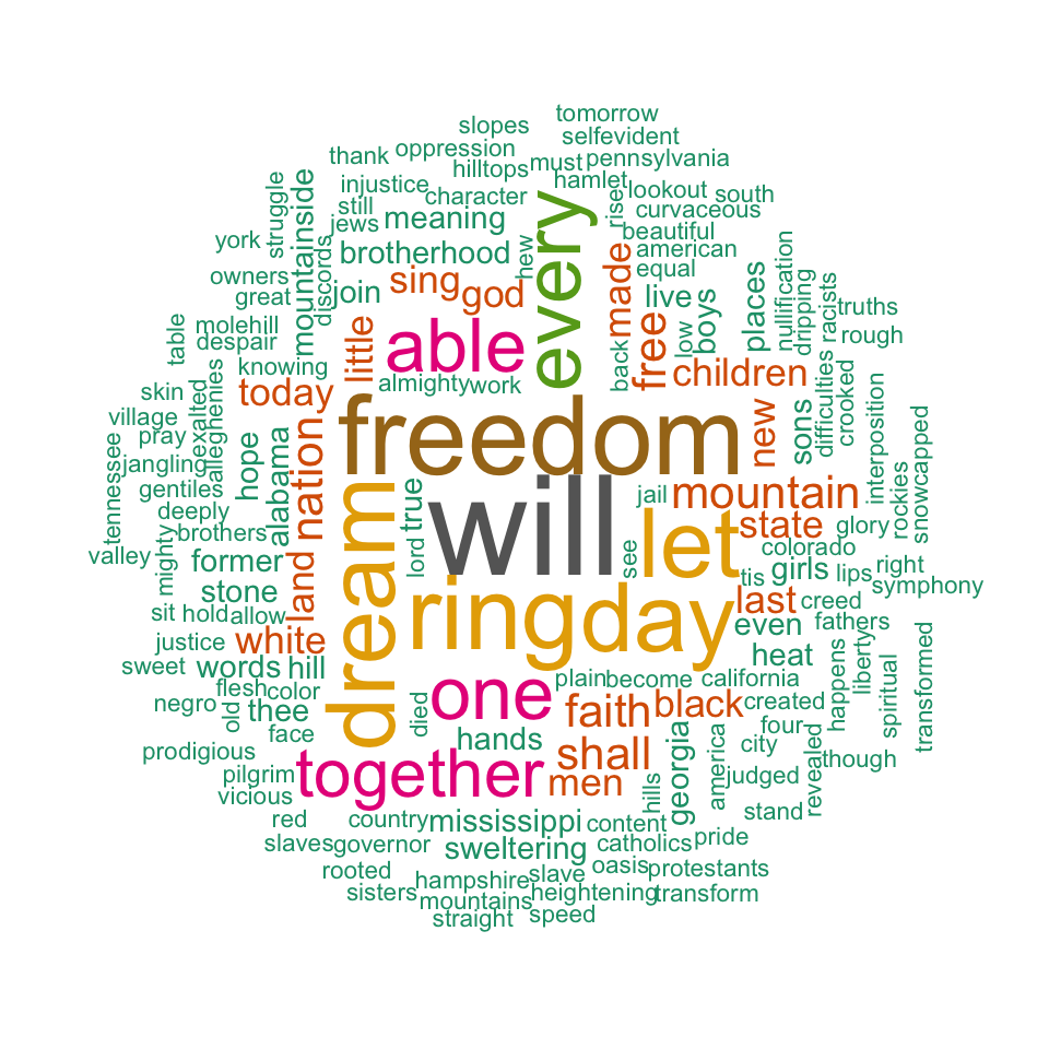
word cloud and text mining, I have a dream speech from Martin Luther King
The above word cloud clearly shows that “Will”, “freedom”, “dream”, “day” and “together” are the five most important words in the “I have a dream speech” from Martin Luther King.
Arguments of the word cloud generator function :
- words : the words to be plotted
- freq : their frequencies
- min.freq : words with frequency below min.freq will not be plotted
- max.words : maximum number of words to be plotted
- random.order : plot words in random order. If false, they will be plotted in decreasing frequency
- rot.per : proportion words with 90 degree rotation (vertical text)
- colors : color words from least to most frequent. Use, for example, colors =“black” for single color.
Go further
Explore frequent terms and their associations
You can have a look at the frequent terms in the term-document matrix as follow. In the example below we want to find words that occur at least four times :
findFreqTerms(dtm, lowfreq = 4) [1] "able" "day" "dream" "every" "faith" "free" "freedom" "let" "mountain" "nation"
[11] "one" "ring" "shall" "together" "will" You can analyze the association between frequent terms (i.e., terms which correlate) using findAssocs() function. The R code below identifies which words are associated with “freedom” in I have a dream speech :
findAssocs(dtm, terms = "freedom", corlimit = 0.3)$freedom
let ring mississippi mountainside stone every mountain state
0.89 0.86 0.34 0.34 0.34 0.32 0.32 0.32 The frequency table of words
head(d, 10) word freq
will will 17
freedom freedom 13
ring ring 12
day day 11
dream dream 11
let let 11
every every 9
able able 8
one one 8
together together 7Plot word frequencies
The frequency of the first 10 frequent words are plotted :
barplot(d[1:10,]$freq, las = 2, names.arg = d[1:10,]$word,
        col ="lightblue", main ="Most frequent words",
        ylab = "Word frequencies")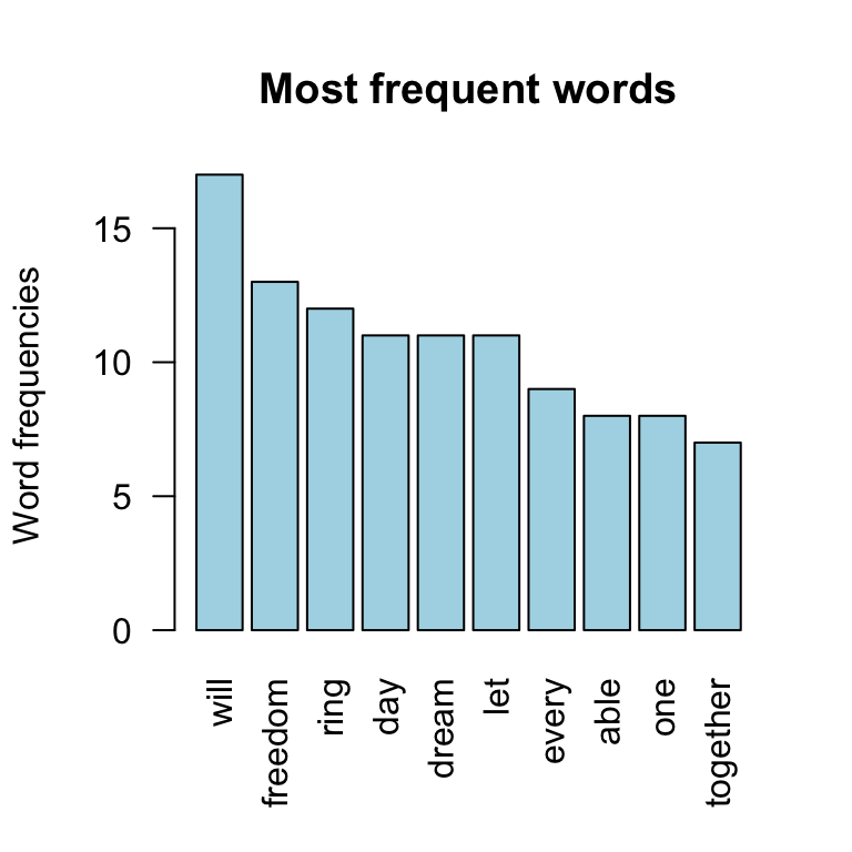
word cloud and text mining
Infos
This analysis has been performed using R (ver. 3.3.2).
Show me some love with the like buttons below... Thank you and please don't forget to share and comment below!!
Montrez-moi un peu d'amour avec les like ci-dessous ... Merci et n'oubliez pas, s'il vous plaît, de partager et de commenter ci-dessous!
Recommended for You!


Recommended for you
This section contains the best data science and self-development resources to help you on your path.
Books - Data Science
Our Books
- Practical Guide to Cluster Analysis in R by A. Kassambara (Datanovia)
- Practical Guide To Principal Component Methods in R by A. Kassambara (Datanovia)
- Machine Learning Essentials: Practical Guide in R by A. Kassambara (Datanovia)
- R Graphics Essentials for Great Data Visualization by A. Kassambara (Datanovia)
- GGPlot2 Essentials for Great Data Visualization in R by A. Kassambara (Datanovia)
- Network Analysis and Visualization in R by A. Kassambara (Datanovia)
- Practical Statistics in R for Comparing Groups: Numerical Variables by A. Kassambara (Datanovia)
- Inter-Rater Reliability Essentials: Practical Guide in R by A. Kassambara (Datanovia)
Others
- R for Data Science: Import, Tidy, Transform, Visualize, and Model Data by Hadley Wickham & Garrett Grolemund
- Hands-On Machine Learning with Scikit-Learn, Keras, and TensorFlow: Concepts, Tools, and Techniques to Build Intelligent Systems by Aurelien Géron
- Practical Statistics for Data Scientists: 50 Essential Concepts by Peter Bruce & Andrew Bruce
- Hands-On Programming with R: Write Your Own Functions And Simulations by Garrett Grolemund & Hadley Wickham
- An Introduction to Statistical Learning: with Applications in R by Gareth James et al.
- Deep Learning with R by François Chollet & J.J. Allaire
- Deep Learning with Python by François Chollet
Click to follow us on Facebook :
Comment this article by clicking on "Discussion" button (top-right position of this page)