


Two-Way ANOVA Test in R
- What is two-way ANOVA test?
- Two-way ANOVA test hypotheses
- Assumptions of two-way ANOVA test
- Compute two-way ANOVA test in R: balanced designs
- Compute two-way ANOVA test in R for unbalanced designs
- See also
- Read more
- Infos
What is two-way ANOVA test?
The grouping variables are also known as factors. The different categories (groups) of a factor are called levels. The number of levels can vary between factors. The level combinations of factors are called cell.
When the sample sizes within cells are equal, we have the so-called balanced design. In this case the standard two-way ANOVA test can be applied.
- When the sample sizes within each level of the independent variables are not the same (case of unbalanced designs), the ANOVA test should be handled differently.
This tutorial describes how to compute two-way ANOVA test in R software for balanced and unbalanced designs.

Two-way ANOVA test hypotheses
- There is no difference in the means of factor A
- There is no difference in means of factor B
- There is no interaction between factors A and B
The alternative hypothesis for cases 1 and 2 is: the means are not equal.
The alternative hypothesis for case 3 is: there is an interaction between A and B.
Assumptions of two-way ANOVA test
Two-way ANOVA, like all ANOVA tests, assumes that the observations within each cell are normally distributed and have equal variances. We’ll show you how to check these assumptions after fitting ANOVA.
Compute two-way ANOVA test in R: balanced designs
Balanced designs correspond to the situation where we have equal sample sizes within levels of our independent grouping levels.
Import your data into R
Prepare your data as specified here: Best practices for preparing your data set for R
Save your data in an external .txt tab or .csv files
Import your data into R as follow:
# If .txt tab file, use this
my_data <- read.delim(file.choose())
# Or, if .csv file, use this
my_data <- read.csv(file.choose())
Here, we’ll use the built-in R data set named ToothGrowth. It contains data from a study evaluating the effect of vitamin C on tooth growth in Guinea pigs. The experiment has been performed on 60 pigs, where each animal received one of three dose levels of vitamin C (0.5, 1, and 2 mg/day) by one of two delivery methods, (orange juice or ascorbic acid (a form of vitamin C and coded as VC). Tooth length was measured and a sample of the data is shown below.
# Store the data in the variable my_data
my_data <- ToothGrowth
Check your data
To get an idea of what the data look like, we display a random sample of the data using the function sample_n()[in dplyr package]. First, install dplyr if you don’t have it:
install.packages("dplyr")# Show a random sample
set.seed(1234)
dplyr::sample_n(my_data, 10) len supp dose
38 9.4 OJ 0.5
36 10.0 OJ 0.5
37 8.2 OJ 0.5
50 27.3 OJ 1.0
59 29.4 OJ 2.0
1 4.2 VC 0.5
13 15.2 VC 1.0
56 30.9 OJ 2.0
27 26.7 VC 2.0
53 22.4 OJ 2.0# Check the structure
str(my_data)'data.frame': 60 obs. of 3 variables:
$ len : num 4.2 11.5 7.3 5.8 6.4 10 11.2 11.2 5.2 7 ...
$ supp: Factor w/ 2 levels "OJ","VC": 2 2 2 2 2 2 2 2 2 2 ...
$ dose: num 0.5 0.5 0.5 0.5 0.5 0.5 0.5 0.5 0.5 0.5 ...From the output above, R considers “dose” as a numeric variable. We’ll convert it as a factor variable (i.e., grouping variable) as follow.
# Convert dose as a factor and recode the levels
# as "D0.5", "D1", "D2"
my_data$dose <- factor(my_data$dose,
                  levels = c(0.5, 1, 2),
                  labels = c("D0.5", "D1", "D2"))
head(my_data)
len supp dose
1 4.2 VC D0.5
2 11.5 VC D0.5
3 7.3 VC D0.5
4 5.8 VC D0.5
5 6.4 VC D0.5
6 10.0 VC D0.5Question: We want to know if tooth length depends on supp and dose.
- Generate frequency tables:
table(my_data$supp, my_data$dose)
     D0.5 D1 D2
  OJ   10 10 10
  VC   10 10 10
We have 2X3 design cells with the factors being supp and dose and 10 subjects in each cell. Here, we have a balanced design. In the next sections I’ll describe how to analyse data from balanced designs, since this is the simplest case.
Visualize your data
Box plots and line plots can be used to visualize group differences:
- Box plot to plot the data grouped by the combinations of the levels of the two factors.
Two-way interaction plot, which plots the mean (or other summary) of the response for two-way combinations of factors, thereby illustrating possible interactions.
To use R base graphs read this: R base graphs. Here, we’ll use the ggpubr R package for an easy ggplot2-based data visualization.
Install the latest version of ggpubr from GitHub as follow (recommended):
# Install
if(!require(devtools)) install.packages("devtools")
devtools::install_github("kassambara/ggpubr")- Or, install from CRAN as follow:
install.packages("ggpubr")- Visualize your data with ggpubr:
# Box plot with multiple groups
# +++++++++++++++++++++
# Plot tooth length ("len") by groups ("dose")
# Color box plot by a second group: "supp"
library("ggpubr")
ggboxplot(my_data, x = "dose", y = "len", color = "supp",
          palette = c("#00AFBB", "#E7B800"))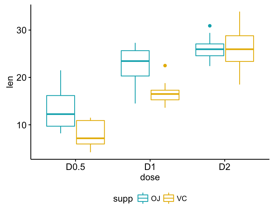
Two-Way ANOVA Test in R
# Line plots with multiple groups
# +++++++++++++++++++++++
# Plot tooth length ("len") by groups ("dose")
# Color box plot by a second group: "supp"
# Add error bars: mean_se
# (other values include: mean_sd, mean_ci, median_iqr, ....)
library("ggpubr")
ggline(my_data, x = "dose", y = "len", color = "supp",
       add = c("mean_se", "dotplot"),
       palette = c("#00AFBB", "#E7B800"))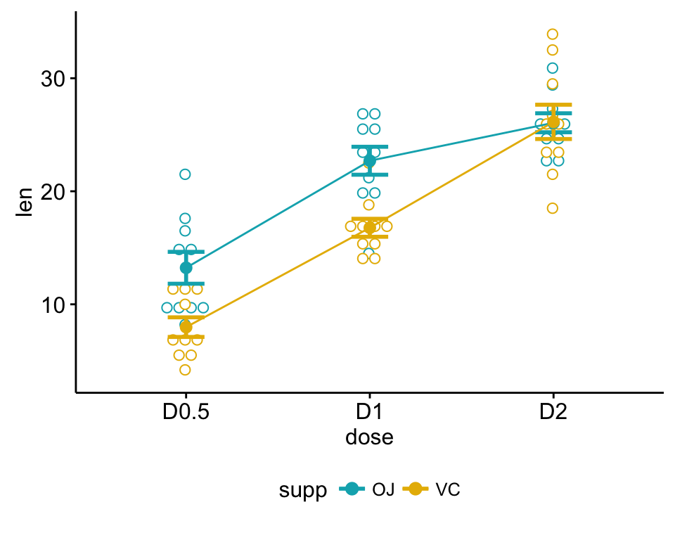
Two-Way ANOVA Test in R
If you still want to use R base graphs, type the following scripts:
# Box plot with two factor variables
boxplot(len ~ supp * dose, data=my_data, frame = FALSE,
        col = c("#00AFBB", "#E7B800"), ylab="Tooth Length")
# Two-way interaction plot
interaction.plot(x.factor = my_data$dose, trace.factor = my_data$supp,
                 response = my_data$len, fun = mean,
                 type = "b", legend = TRUE,
                 xlab = "Dose", ylab="Tooth Length",
                 pch=c(1,19), col = c("#00AFBB", "#E7B800"))
Arguments used for the function interaction.plot():
- x.factor: the factor to be plotted on x axis.
- trace.factor: the factor to be plotted as lines
- response: a numeric variable giving the response
- type: the type of plot. Allowed values include p (for point only), l (for line only) and b (for both point and line).
Compute two-way ANOVA test
We want to know if tooth length depends on supp and dose.
The R function aov() can be used to answer this question. The function summary.aov() is used to summarize the analysis of variance model.
res.aov2 <- aov(len ~ supp + dose, data = my_data)
summary(res.aov2)
Df Sum Sq Mean Sq F value Pr(>F)
supp 1 205.4 205.4 14.02 0.000429 ***
dose 2 2426.4 1213.2 82.81 < 2e-16 ***
Residuals 56 820.4 14.7
---
Signif. codes: 0 '***' 0.001 '**' 0.01 '*' 0.05 '.' 0.1 ' ' 1The output includes the columns F value and Pr(>F) corresponding to the p-value of the test.
From the ANOVA table we can conclude that both supp and dose are statistically significant. dose is the most significant factor variable. These results would lead us to believe that changing delivery methods (supp) or the dose of vitamin C, will impact significantly the mean tooth length.
Not the above fitted model is called additive model. It makes an assumption that the two factor variables are independent. If you think that these two variables might interact to create an synergistic effect, replace the plus symbol (+) by an asterisk (*), as follow.
# Two-way ANOVA with interaction effect
# These two calls are equivalent
res.aov3 <- aov(len ~ supp * dose, data = my_data)
res.aov3 <- aov(len ~ supp + dose + supp:dose, data = my_data)
summary(res.aov3)
Df Sum Sq Mean Sq F value Pr(>F)
supp 1 205.4 205.4 15.572 0.000231 ***
dose 2 2426.4 1213.2 92.000 < 2e-16 ***
supp:dose 2 108.3 54.2 4.107 0.021860 *
Residuals 54 712.1 13.2
---
Signif. codes: 0 '***' 0.001 '**' 0.01 '*' 0.05 '.' 0.1 ' ' 1It can be seen that the two main effects (supp and dose) are statistically significant, as well as their interaction.
Note that, in the situation where the interaction is not significant you should use the additive model.
Interpret the results
From the ANOVA results, you can conclude the following, based on the p-values and a significance level of 0.05:
- the p-value of supp is 0.000429 (significant), which indicates that the levels of supp are associated with significant different tooth length.
- the p-value of dose is < 2e-16 (significant), which indicates that the levels of dose are associated with significant different tooth length.
- the p-value for the interaction between supp*dose is 0.02 (significant), which indicates that the relationships between dose and tooth length depends on the supp method.
Compute some summary statistics
- Compute mean and SD by groups using dplyr R package:
require("dplyr")
group_by(my_data, supp, dose) %>%
  summarise(
    count = n(),
    mean = mean(len, na.rm = TRUE),
    sd = sd(len, na.rm = TRUE)
  )
Source: local data frame [6 x 5]
Groups: supp [?]
supp dose count mean sd
(fctr) (fctr) (int) (dbl) (dbl)
1 OJ D0.5 10 13.23 4.459709
2 OJ D1 10 22.70 3.910953
3 OJ D2 10 26.06 2.655058
4 VC D0.5 10 7.98 2.746634
5 VC D1 10 16.77 2.515309
6 VC D2 10 26.14 4.797731- It’s also possible to use the function model.tables() as follow:
model.tables(res.aov3, type="means", se = TRUE)Multiple pairwise-comparison between the means of groups
In ANOVA test, a significant p-value indicates that some of the group means are different, but we don’t know which pairs of groups are different.
It’s possible to perform multiple pairwise-comparison, to determine if the mean difference between specific pairs of group are statistically significant.
Tukey multiple pairwise-comparisons
As the ANOVA test is significant, we can compute Tukey HSD (Tukey Honest Significant Differences, R function: TukeyHSD()) for performing multiple pairwise-comparison between the means of groups. The function TukeyHD() takes the fitted ANOVA as an argument.
We don’t need to perform the test for the “supp” variable because it has only two levels, which have been already proven to be significantly different by ANOVA test. Therefore, the Tukey HSD test will be done only for the factor variable “dose”.
TukeyHSD(res.aov3, which = "dose") Tukey multiple comparisons of means
95% family-wise confidence level
Fit: aov(formula = len ~ supp + dose + supp:dose, data = my_data)
$dose
diff lwr upr p adj
D1-D0.5 9.130 6.362488 11.897512 0.0e+00
D2-D0.5 15.495 12.727488 18.262512 0.0e+00
D2-D1 6.365 3.597488 9.132512 2.7e-06- diff: difference between means of the two groups
- lwr, upr: the lower and the upper end point of the confidence interval at 95% (default)
- p adj: p-value after adjustment for the multiple comparisons.
It can be seen from the output, that all pairwise comparisons are significant with an adjusted p-value < 0.05.
Multiple comparisons using multcomp package
It’s possible to use the function glht() [in multcomp package] to perform multiple comparison procedures for an ANOVA. glht stands for general linear hypothesis tests. The simplified format is as follow:
glht(model, lincft)- model: a fitted model, for example an object returned by aov().
- lincft(): a specification of the linear hypotheses to be tested. Multiple comparisons in ANOVA models are specified by objects returned from the function mcp().
Use glht() to perform multiple pairwise-comparisons:
library(multcomp)
summary(glht(res.aov2, linfct = mcp(dose = "Tukey")))
     Simultaneous Tests for General Linear Hypotheses
Multiple Comparisons of Means: Tukey Contrasts
Fit: aov(formula = len ~ supp + dose, data = my_data)
Linear Hypotheses:
               Estimate Std. Error t value Pr(>|t|)
D1 - D0.5 == 0    9.130      1.210   7.543   <1e-05 ***
D2 - D0.5 == 0   15.495      1.210  12.802   <1e-05 ***
D2 - D1 == 0      6.365      1.210   5.259   <1e-05 ***
---
Signif. codes:  0 '***' 0.001 '**' 0.01 '*' 0.05 '.' 0.1 ' ' 1
(Adjusted p values reported -- single-step method)
Pairwise t-test
The function pairwise.t.test() can be also used to calculate pairwise comparisons between group levels with corrections for multiple testing.
pairwise.t.test(my_data$len, my_data$dose,
                p.adjust.method = "BH")
    Pairwise comparisons using t tests with pooled SD
data:  my_data$len and my_data$dose
   D0.5    D1
D1 1.0e-08 -
D2 4.4e-16 1.4e-05
P value adjustment method: BH
Check ANOVA assumptions: test validity?
ANOVA assumes that the data are normally distributed and the variance across groups are homogeneous. We can check that with some diagnostic plots.
Check the homogeneity of variance assumption
The residuals versus fits plot is used to check the homogeneity of variances. In the plot below, there is no evident relationships between residuals and fitted values (the mean of each groups), which is good. So, we can assume the homogeneity of variances.
# 1. Homogeneity of variances
plot(res.aov3, 1)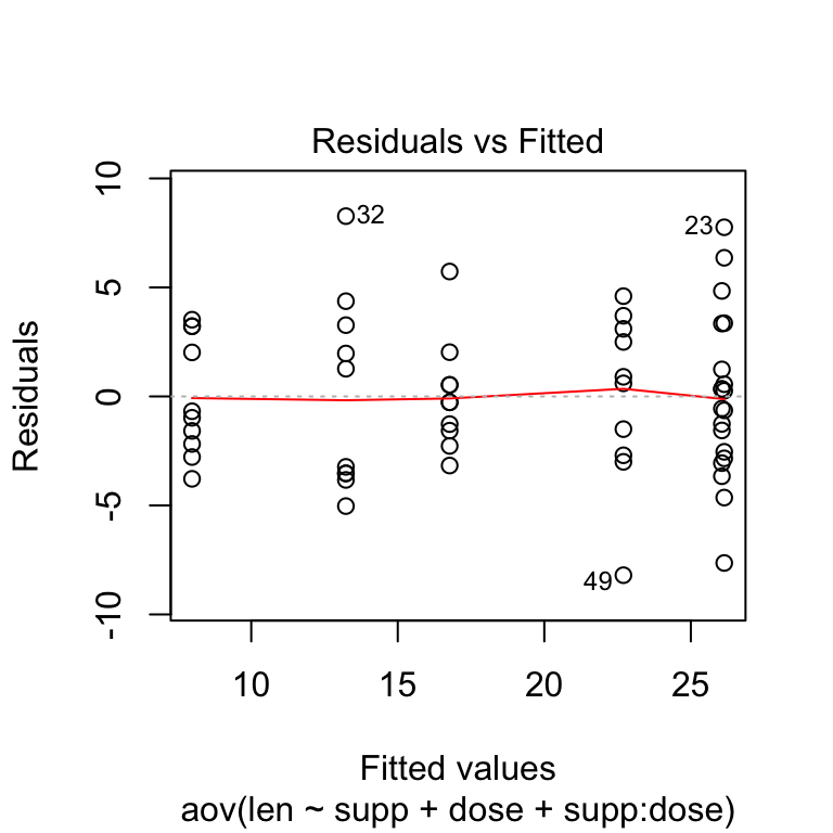
Two-Way ANOVA Test in R
Points 32 and 23 are detected as outliers, which can severely affect normality and homogeneity of variance. It can be useful to remove outliers to meet the test assumptions.
Use the Levene’s test to check the homogeneity of variances. The function leveneTest() [in car package] will be used:
library(car)
leveneTest(len ~ supp*dose, data = my_data)
Levene's Test for Homogeneity of Variance (center = median)
Df F value Pr(>F)
group 5 1.7086 0.1484
54 From the output above we can see that the p-value is not less than the significance level of 0.05. This means that there is no evidence to suggest that the variance across groups is statistically significantly different. Therefore, we can assume the homogeneity of variances in the different treatment groups.
Check the normality assumpttion
Normality plot of the residuals. In the plot below, the quantiles of the residuals are plotted against the quantiles of the normal distribution. A 45-degree reference line is also plotted.
The normal probability plot of residuals is used to verify the assumption that the residuals are normally distributed.
The normal probability plot of the residuals should approximately follow a straight line.
# 2. Normality
plot(res.aov3, 2)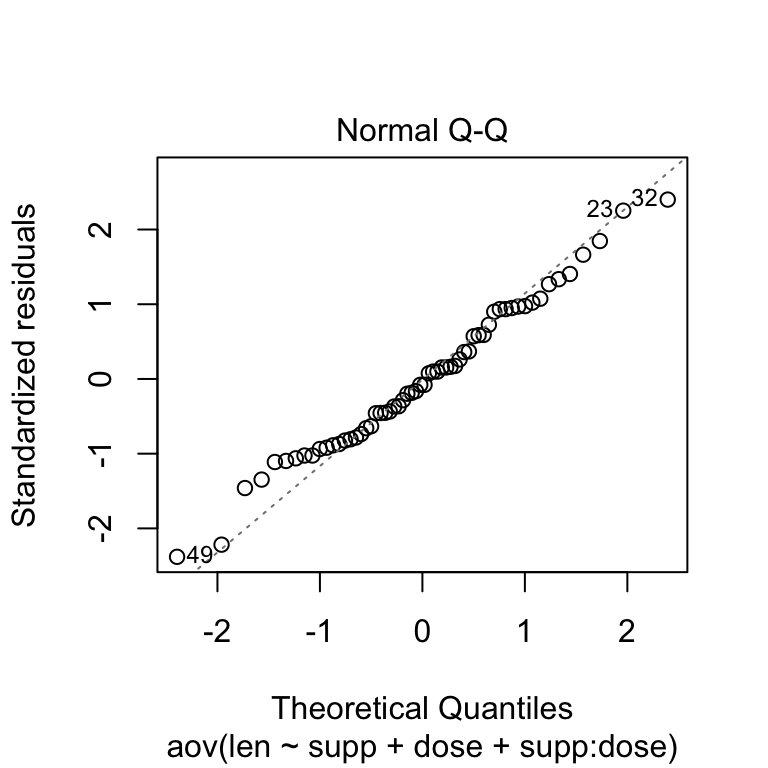
Two-Way ANOVA Test in R
As all the points fall approximately along this reference line, we can assume normality.
The conclusion above, is supported by the Shapiro-Wilk test on the ANOVA residuals (W = 0.98, p = 0.5) which finds no indication that normality is violated.
# Extract the residuals
aov_residuals <- residuals(object = res.aov3)
# Run Shapiro-Wilk test
shapiro.test(x = aov_residuals )
    Shapiro-Wilk normality test
data:  aov_residuals
W = 0.98499, p-value = 0.6694
Compute two-way ANOVA test in R for unbalanced designs
An unbalanced design has unequal numbers of subjects in each group.
There are three fundamentally different ways to run an ANOVA in an unbalanced design. They are known as Type-I, Type-II and Type-III sums of squares. To keep things simple, note that The recommended method are the Type-III sums of squares.
The three methods give the same result when the design is balanced. However, when the design is unbalanced, they don’t give the same results.
The function Anova() [in car package] can be used to compute two-way ANOVA test for unbalanced designs.
First install the package on your computer. In R, type install.packages(“car”). Then:
library(car)
my_anova <- aov(len ~ supp * dose, data = my_data)
Anova(my_anova, type = "III")
Anova Table (Type III tests)
Response: len
Sum Sq Df F value Pr(>F)
(Intercept) 1750.33 1 132.730 3.603e-16 ***
supp 137.81 1 10.450 0.002092 **
dose 885.26 2 33.565 3.363e-10 ***
supp:dose 108.32 2 4.107 0.021860 *
Residuals 712.11 54
---
Signif. codes: 0 '***' 0.001 '**' 0.01 '*' 0.05 '.' 0.1 ' ' 1See also
- Analysis of variance (ANOVA, parametric):
- Kruskal-Wallis Test in R (non parametric alternative to one-way ANOVA)
Infos
This analysis has been performed using R software (ver. 3.2.4).
Show me some love with the like buttons below... Thank you and please don't forget to share and comment below!!
Montrez-moi un peu d'amour avec les like ci-dessous ... Merci et n'oubliez pas, s'il vous plaît, de partager et de commenter ci-dessous!
Recommended for You!


Recommended for you
This section contains the best data science and self-development resources to help you on your path.
Books - Data Science
Our Books
- Practical Guide to Cluster Analysis in R by A. Kassambara (Datanovia)
- Practical Guide To Principal Component Methods in R by A. Kassambara (Datanovia)
- Machine Learning Essentials: Practical Guide in R by A. Kassambara (Datanovia)
- R Graphics Essentials for Great Data Visualization by A. Kassambara (Datanovia)
- GGPlot2 Essentials for Great Data Visualization in R by A. Kassambara (Datanovia)
- Network Analysis and Visualization in R by A. Kassambara (Datanovia)
- Practical Statistics in R for Comparing Groups: Numerical Variables by A. Kassambara (Datanovia)
- Inter-Rater Reliability Essentials: Practical Guide in R by A. Kassambara (Datanovia)
Others
- R for Data Science: Import, Tidy, Transform, Visualize, and Model Data by Hadley Wickham & Garrett Grolemund
- Hands-On Machine Learning with Scikit-Learn, Keras, and TensorFlow: Concepts, Tools, and Techniques to Build Intelligent Systems by Aurelien Géron
- Practical Statistics for Data Scientists: 50 Essential Concepts by Peter Bruce & Andrew Bruce
- Hands-On Programming with R: Write Your Own Functions And Simulations by Garrett Grolemund & Hadley Wickham
- An Introduction to Statistical Learning: with Applications in R by Gareth James et al.
- Deep Learning with R by François Chollet & J.J. Allaire
- Deep Learning with Python by François Chollet
Click to follow us on Facebook :
Comment this article by clicking on "Discussion" button (top-right position of this page)