


Correlation Test Between Two Variables in R
What is correlation test?
For instance, if we are interested to know whether there is a relationship between the heights of fathers and sons, a correlation coefficient can be calculated to answer this question.
If there is no relationship between the two variables (father and son heights), the average height of son should be the same regardless of the height of the fathers and vice versa.
Here, we’ll describe the different correlation methods and we’ll provide pratical examples using R software.
Install and load required R packages
We’ll use the ggpubr R package for an easy ggplot2-based data visualization
- Install the latest version from GitHub as follow (recommended):
if(!require(devtools)) install.packages("devtools")
devtools::install_github("kassambara/ggpubr")- Or, install from CRAN as follow:
install.packages("ggpubr")- Load ggpubr as follow:
library("ggpubr")Methods for correlation analyses
There are different methods to perform correlation analysis:
Pearson correlation (r), which measures a linear dependence between two variables (x and y). It’s also known as a parametric correlation test because it depends to the distribution of the data. It can be used only when x and y are from normal distribution. The plot of y = f(x) is named the linear regression curve.
Kendall tau and Spearman rho, which are rank-based correlation coefficients (non-parametric)
The most commonly used method is the Pearson correlation method.
Correlation formula
In the formula below,
- x and y are two vectors of length n
- \(m_x\) and \(m_y\) corresponds to the means of x and y, respectively.
Pearson correlation formula
\[ r = \frac{\sum{(x-m_x)(y-m_y)}}{\sqrt{\sum{(x-m_x)^2}\sum{(y-m_y)^2}}} \]
\(m_x\) and \(m_y\) are the means of x and y variables.
The p-value (significance level) of the correlation can be determined :
by using the correlation coefficient table for the degrees of freedom : \(df = n-2\), where \(n\) is the number of observation in x and y variables.
or by calculating the t value as follow:
\[ t = \frac{r}{\sqrt{1-r^2}}\sqrt{n-2} \]
In the case 2) the corresponding p-value is determined using t distribution table for \(df = n-2\)
If the p-value is < 5%, then the correlation between x and y is significant.
Spearman correlation formula
The Spearman correlation method computes the correlation between the rank of x and the rank of y variables.
\[ rho = \frac{\sum(x' - m_{x'})(y'_i - m_{y'})}{\sqrt{\sum(x' - m_{x'})^2 \sum(y' - m_{y'})^2}} \]
Where \(x' = rank(x_)\) and \(y' = rank(y)\).
Kendall correlation formula
The Kendall correlation method measures the correspondence between the ranking of x and y variables. The total number of possible pairings of x with y observations is \(n(n-1)/2\), where n is the size of x and y.
The procedure is as follow:
Begin by ordering the pairs by the x values. If x and y are correlated, then they would have the same relative rank orders.
Now, for each \(y_i\), count the number of \(y_j > y_i\) (concordant pairs (c)) and the number of \(y_j < y_i\) (discordant pairs (d)).
Kendall correlation distance is defined as follow:
\[ tau = \frac{n_c - n_d}{\frac{1}{2}n(n-1)} \]
Where,
- \(n_c\): total number of concordant pairs
- \(n_d\): total number of discordant pairs
- \(n\): size of x and y
Compute correlation in R
R functions
Correlation coefficient can be computed using the functions cor() or cor.test():
- cor() computes the correlation coefficient
- cor.test() test for association/correlation between paired samples. It returns both the correlation coefficient and the significance level(or p-value) of the correlation .
The simplified formats are:
cor(x, y, method = c("pearson", "kendall", "spearman"))
cor.test(x, y, method=c("pearson", "kendall", "spearman"))- x, y: numeric vectors with the same length
- method: correlation method
If your data contain missing values, use the following R code to handle missing values by case-wise deletion.
cor(x, y, method = "pearson", use = "complete.obs")Import your data into R
Prepare your data as specified here: Best practices for preparing your data set for R
Save your data in an external .txt tab or .csv files
Import your data into R as follow:
# If .txt tab file, use this
my_data <- read.delim(file.choose())
# Or, if .csv file, use this
my_data <- read.csv(file.choose())
Here, we’ll use the built-in R data set mtcars as an example.
The R code below computes the correlation between mpg and wt variables in mtcars data set:
my_data <- mtcars
head(my_data, 6)
mpg cyl disp hp drat wt qsec vs am gear carb
Mazda RX4 21.0 6 160 110 3.90 2.620 16.46 0 1 4 4
Mazda RX4 Wag 21.0 6 160 110 3.90 2.875 17.02 0 1 4 4
Datsun 710 22.8 4 108 93 3.85 2.320 18.61 1 1 4 1
Hornet 4 Drive 21.4 6 258 110 3.08 3.215 19.44 1 0 3 1
Hornet Sportabout 18.7 8 360 175 3.15 3.440 17.02 0 0 3 2
Valiant 18.1 6 225 105 2.76 3.460 20.22 1 0 3 1We want to compute the correlation between mpg and wt variables.
Visualize your data using scatter plots
To use R base graphs, click this link: scatter plot - R base graphs. Here, we’ll use the ggpubr R package.
library("ggpubr")
ggscatter(my_data, x = "mpg", y = "wt",
          add = "reg.line", conf.int = TRUE,
          cor.coef = TRUE, cor.method = "pearson",
          xlab = "Miles/(US) gallon", ylab = "Weight (1000 lbs)")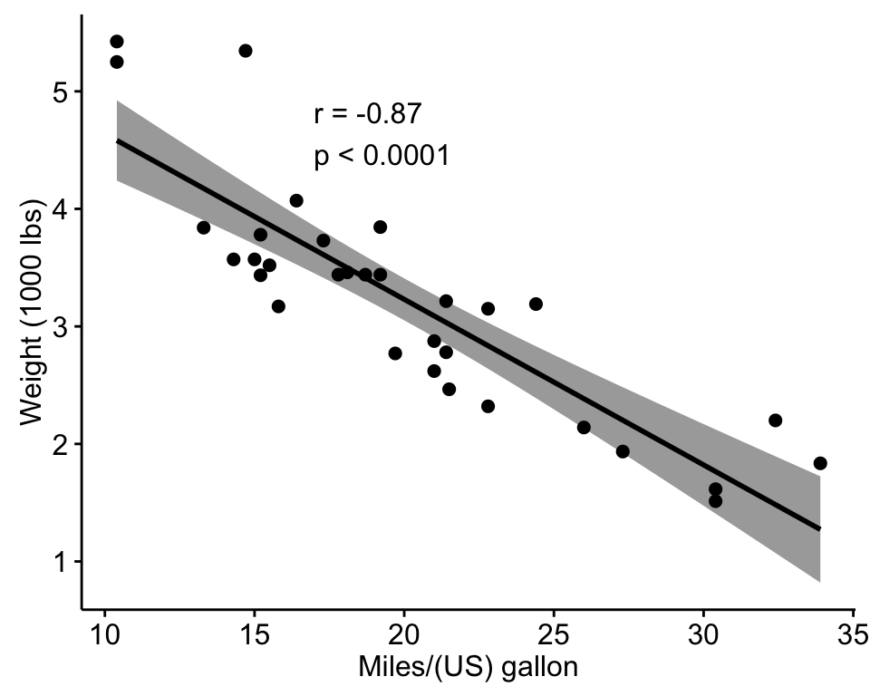
Correlation Test Between Two Variables in R software
Preleminary test to check the test assumptions
Is the covariation linear? Yes, form the plot above, the relationship is linear. In the situation where the scatter plots show curved patterns, we are dealing with nonlinear association between the two variables.
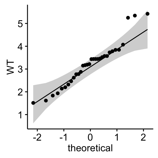
- Are the data from each of the 2 variables (x, y) follow a normal distribution?
- Use Shapiro-Wilk normality test –> R function: shapiro.test()
- and look at the normality plot —> R function: ggpubr::ggqqplot()
- Shapiro-Wilk test can be performed as follow:
- Null hypothesis: the data are normally distributed
- Alternative hypothesis: the data are not normally distributed
# Shapiro-Wilk normality test for mpg
shapiro.test(my_data$mpg) # => p = 0.1229
# Shapiro-Wilk normality test for wt
shapiro.test(my_data$wt) # => p = 0.09
From the output, the two p-values are greater than the significance level 0.05 implying that the distribution of the data are not significantly different from normal distribution. In other words, we can assume the normality.
- Visual inspection of the data normality using Q-Q plots (quantile-quantile plots). Q-Q plot draws the correlation between a given sample and the normal distribution.
library("ggpubr")
# mpg
ggqqplot(my_data$mpg, ylab = "MPG")
# wt
ggqqplot(my_data$wt, ylab = "WT")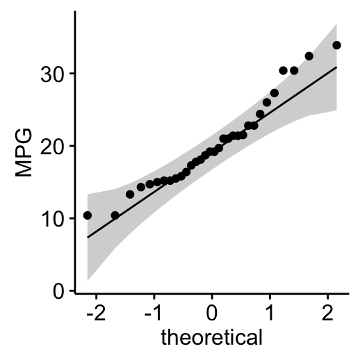
Correlation Test Between Two Variables in R software
From the normality plots, we conclude that both populations may come from normal distributions.
Note that, if the data are not normally distributed, it’s recommended to use the non-parametric correlation, including Spearman and Kendall rank-based correlation tests.
Pearson correlation test
Correlation test between mpg and wt variables:
res <- cor.test(my_data$wt, my_data$mpg,
                    method = "pearson")
res
    Pearson's product-moment correlation
data:  my_data$wt and my_data$mpg
t = -9.559, df = 30, p-value = 1.294e-10
alternative hypothesis: true correlation is not equal to 0
95 percent confidence interval:
 -0.9338264 -0.7440872
sample estimates:
       cor
-0.8676594
In the result above :
- t is the t-test statistic value (t = -9.559),
- df is the degrees of freedom (df= 30),
- p-value is the significance level of the t-test (p-value = 1.29410^{-10}).
- conf.int is the confidence interval of the correlation coefficient at 95% (conf.int = [-0.9338, -0.7441]);
- sample estimates is the correlation coefficient (Cor.coeff = -0.87).
Interpretation of the result
The p-value of the test is 1.29410^{-10}, which is less than the significance level alpha = 0.05. We can conclude that wt and mpg are significantly correlated with a correlation coefficient of -0.87 and p-value of 1.29410^{-10} .
Access to the values returned by cor.test() function
The function cor.test() returns a list containing the following components:
- p.value: the p-value of the test
- estimate: the correlation coefficient
# Extract the p.value
res$p.value
[1] 1.293959e-10# Extract the correlation coefficient
res$estimate cor
-0.8676594 Kendall rank correlation test
The Kendall rank correlation coefficient or Kendall’s tau statistic is used to estimate a rank-based measure of association. This test may be used if the data do not necessarily come from a bivariate normal distribution.
res2 <- cor.test(my_data$wt, my_data$mpg,  method="kendall")
res2
    Kendall's rank correlation tau
data:  my_data$wt and my_data$mpg
z = -5.7981, p-value = 6.706e-09
alternative hypothesis: true tau is not equal to 0
sample estimates:
       tau
-0.7278321
tau is the Kendall correlation coefficient.
The correlation coefficient between x and y are -0.7278 and the p-value is 6.70610^{-9}.
Spearman rank correlation coefficient
Spearman’s rho statistic is also used to estimate a rank-based measure of association. This test may be used if the data do not come from a bivariate normal distribution.
res2 <-cor.test(my_data$wt, my_data$mpg,  method = "spearman")
res2
    Spearman's rank correlation rho
data:  my_data$wt and my_data$mpg
S = 10292, p-value = 1.488e-11
alternative hypothesis: true rho is not equal to 0
sample estimates:
      rho
-0.886422
rho is the Spearman’s correlation coefficient.
The correlation coefficient between x and y are -0.8864 and the p-value is 1.48810^{-11}.
Interpret correlation coefficient
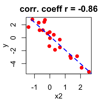
Correlation coefficient is comprised between -1 and 1:
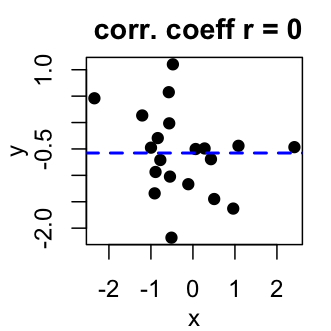
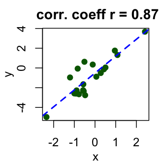
- -1 indicates a strong negative correlation : this means that every time x increases, y decreases (left panel figure)
- 0 means that there is no association between the two variables (x and y) (middle panel figure)
- 1 indicates a strong positive correlation : this means that y increases with x (right panel figure)
Correlation Test Between Two Variables in R software
Online correlation coefficient calculator
You can compute correlation test between two variables, online, without any installation by clicking the following link:
Summary
- Use the function cor.test(x,y) to analyze the correlation coefficient between two variables and to get significance level of the correlation.
- Three possible correlation methods using the function cor.test(x,y): pearson, kendall, spearman
Infos
This analysis has been performed using R software (ver. 3.2.4).
Show me some love with the like buttons below... Thank you and please don't forget to share and comment below!!
Montrez-moi un peu d'amour avec les like ci-dessous ... Merci et n'oubliez pas, s'il vous plaît, de partager et de commenter ci-dessous!
Recommended for You!


Recommended for you
This section contains the best data science and self-development resources to help you on your path.
Books - Data Science
Our Books
- Practical Guide to Cluster Analysis in R by A. Kassambara (Datanovia)
- Practical Guide To Principal Component Methods in R by A. Kassambara (Datanovia)
- Machine Learning Essentials: Practical Guide in R by A. Kassambara (Datanovia)
- R Graphics Essentials for Great Data Visualization by A. Kassambara (Datanovia)
- GGPlot2 Essentials for Great Data Visualization in R by A. Kassambara (Datanovia)
- Network Analysis and Visualization in R by A. Kassambara (Datanovia)
- Practical Statistics in R for Comparing Groups: Numerical Variables by A. Kassambara (Datanovia)
- Inter-Rater Reliability Essentials: Practical Guide in R by A. Kassambara (Datanovia)
Others
- R for Data Science: Import, Tidy, Transform, Visualize, and Model Data by Hadley Wickham & Garrett Grolemund
- Hands-On Machine Learning with Scikit-Learn, Keras, and TensorFlow: Concepts, Tools, and Techniques to Build Intelligent Systems by Aurelien Géron
- Practical Statistics for Data Scientists: 50 Essential Concepts by Peter Bruce & Andrew Bruce
- Hands-On Programming with R: Write Your Own Functions And Simulations by Garrett Grolemund & Hadley Wickham
- An Introduction to Statistical Learning: with Applications in R by Gareth James et al.
- Deep Learning with R by François Chollet & J.J. Allaire
- Deep Learning with Python by François Chollet
Click to follow us on Facebook :
Comment this article by clicking on "Discussion" button (top-right position of this page)