


Paired Samples T-test in R
What is paired samples t-test?
As an example of data, 20 mice received a treatment X during 3 months. We want to know whether the treatment X has an impact on the weight of the mice.
To answer to this question, the weight of the 20 mice has been measured before and after the treatment. This gives us 20 sets of values before treatment and 20 sets of values after treatment from measuring twice the weight of the same mice.
In such situations, paired t-test can be used to compare the mean weights before and after treatment.
Paired t-test analysis is performed as follow:
- Calculate the difference (\(d\)) between each pair of value
- Compute the mean (\(m\)) and the standard deviation (\(s\)) of \(d\)
- Compare the average difference to 0. If there is any significant difference between the two pairs of samples, then the mean of d (\(m\)) is expected to be far from 0.
Paired t-test can be used only when the difference \(d\) is normally distributed. This can be checked using Shapiro-Wilk test.
Research questions and statistical hypotheses
Typical research questions are:
- whether the mean difference (\(m\)) is equal to 0?
- whether the mean difference (\(m\)) is less than 0?
- whether the mean difference (\(m\)) is greather than 0?
In statistics, we can define the corresponding null hypothesis (\(H_0\)) as follow:
- \(H_0: m = 0\)
- \(H_0: m \leq 0\)
- \(H_0: m \geq 0\)
The corresponding alternative hypotheses (\(H_a\)) are as follow:
- \(H_a: m \ne 0\) (different)
- \(H_a: m > 0\) (greater)
- \(H_a: m < 0\) (less)
Note that:
- Hypotheses 1) are called two-tailed tests
- Hypotheses 2) and 3) are called one-tailed tests
Formula of paired samples t-test
t-test statistisc value can be calculated using the following formula:
\[ t = \frac{m}{s/\sqrt{n}} \]
where,
- m is the mean differences
- n is the sample size (i.e., size of d).
- s is the standard deviation of d
We can compute the p-value corresponding to the absolute value of the t-test statistics (|t|) for the degrees of freedom (df): \(df = n - 1\).
If the p-value is inferior or equal to 0.05, we can conclude that the difference between the two paired samples are significantly different.
Visualize your data and compute paired t-test in R
R function to compute paired t-test
To perform paired samples t-test comparing the means of two paired samples (x & y), the R function t.test() can be used as follow:
t.test(x, y, paired = TRUE, alternative = "two.sided")- x,y: numeric vectors
- paired: a logical value specifying that we want to compute a paired t-test
- alternative: the alternative hypothesis. Allowed value is one of “two.sided” (default), “greater” or “less”.
Import your data into R
Prepare your data as specified here: Best practices for preparing your data set for R
Save your data in an external .txt tab or .csv files
Import your data into R as follow:
# If .txt tab file, use this
my_data <- read.delim(file.choose())
# Or, if .csv file, use this
my_data <- read.csv(file.choose())
Here, we’ll use an example data set, which contains the weight of 10 mice before and after the treatment.
# Data in two numeric vectors
# ++++++++++++++++++++++++++
# Weight of the mice before treatment
before <-c(200.1, 190.9, 192.7, 213, 241.4, 196.9, 172.2, 185.5, 205.2, 193.7)
# Weight of the mice after treatment
after <-c(392.9, 393.2, 345.1, 393, 434, 427.9, 422, 383.9, 392.3, 352.2)
# Create a data frame
my_data <- data.frame(
                group = rep(c("before", "after"), each = 10),
                weight = c(before,  after)
                )
We want to know, if there is any significant difference in the mean weights after treatment?
Check your data
# Print all data
print(my_data)
group weight
1 before 200.1
2 before 190.9
3 before 192.7
4 before 213.0
5 before 241.4
6 before 196.9
7 before 172.2
8 before 185.5
9 before 205.2
10 before 193.7
11 after 392.9
12 after 393.2
13 after 345.1
14 after 393.0
15 after 434.0
16 after 427.9
17 after 422.0
18 after 383.9
19 after 392.3
20 after 352.2Compute summary statistics (mean and sd) by groups using the dplyr package.
- To install dplyr package, type this:
install.packages("dplyr")- Compute summary statistics by groups:
library("dplyr")
group_by(my_data, group) %>%
  summarise(
    count = n(),
    mean = mean(weight, na.rm = TRUE),
    sd = sd(weight, na.rm = TRUE)
  )
Source: local data frame [2 x 4]
group count mean sd
(fctr) (int) (dbl) (dbl)
1 after 10 393.65 29.39801
2 before 10 199.16 18.47354Visualize your data using box plots
To use R base graphs read this: R base graphs. Here, we’ll use the ggpubr R package for an easy ggplot2-based data visualization.
- Install the latest version of ggpubr from GitHub as follow (recommended):
# Install
if(!require(devtools)) install.packages("devtools")
devtools::install_github("kassambara/ggpubr")- Or, install from CRAN as follow:
install.packages("ggpubr")- Visualize your data:
# Plot weight by group and color by group
library("ggpubr")
ggboxplot(my_data, x = "group", y = "weight",
          color = "group", palette = c("#00AFBB", "#E7B800"),
          order = c("before", "after"),
          ylab = "Weight", xlab = "Groups")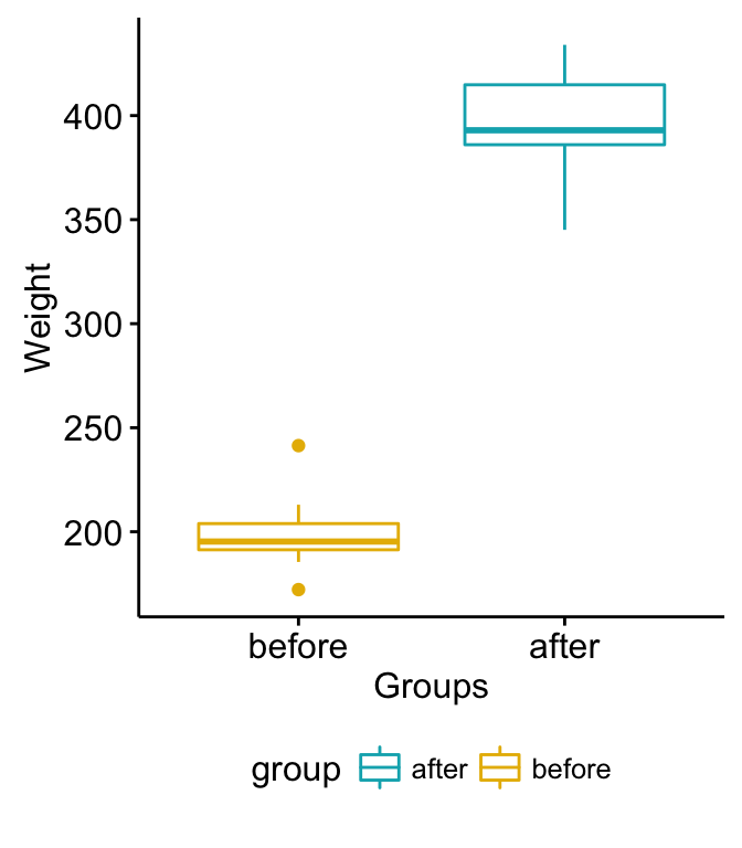
Paired Samples T-test in R
Box plots show you the increase, but lose the paired information. You can use the function plot.paired() [in pairedData package] to plot paired data (“before - after” plot).
- Install pairedData package:
install.packages("PairedData")- Plot paired data:
# Subset weight data before treatment
before <- subset(my_data,  group == "before", weight,
                 drop = TRUE)
# subset weight data after treatment
after <- subset(my_data,  group == "after", weight,
                 drop = TRUE)
# Plot paired data
library(PairedData)
pd <- paired(before, after)
plot(pd, type = "profile") + theme_bw()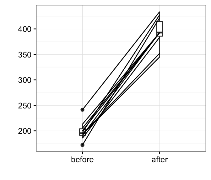
Paired Samples T-test in R
Preleminary test to check paired t-test assumptions
Assumption 1: Are the two samples paired?
Yes, since the data have been collected from measuring twice the weight of the same mice.
Assumption 2: Is this a large sample?
No, because n < 30. Since the sample size is not large enough (less than 30), we need to check whether the differences of the pairs follow a normal distribution.
How to check the normality?
Use Shapiro-Wilk normality test as described at: Normality Test in R.
- Null hypothesis: the data are normally distributed
- Alternative hypothesis: the data are not normally distributed
# compute the difference
d <- with(my_data,
        weight[group == "before"] - weight[group == "after"])
# Shapiro-Wilk normality test for the differences
shapiro.test(d) # => p-value = 0.6141
From the output, the p-value is greater than the significance level 0.05 implying that the distribution of the differences (d) are not significantly different from normal distribution. In other words, we can assume the normality.
Note that, if the data are not normally distributed, it’s recommended to use the non parametric paired two-samples Wilcoxon test.
Compute paired samples t-test
Question : Is there any significant changes in the weights of mice after treatment?
1) Compute paired t-test - Method 1: The data are saved in two different numeric vectors.
# Compute t-test
res <- t.test(before, after, paired = TRUE)
res
    Paired t-test
data:  before and after
t = -20.883, df = 9, p-value = 6.2e-09
alternative hypothesis: true difference in means is not equal to 0
95 percent confidence interval:
 -215.5581 -173.4219
sample estimates:
mean of the differences
                -194.49
2) Compute paired t-test - Method 2: The data are saved in a data frame.
# Compute t-test
res <- t.test(weight ~ group, data = my_data, paired = TRUE)
res
    Paired t-test
data:  weight by group
t = 20.883, df = 9, p-value = 6.2e-09
alternative hypothesis: true difference in means is not equal to 0
95 percent confidence interval:
 173.4219 215.5581
sample estimates:
mean of the differences
                 194.49
As you can see, the two methods give the same results.
In the result above :
- t is the t-test statistic value (t = 20.88),
- df is the degrees of freedom (df= 9),
- p-value is the significance level of the t-test (p-value = 6.210^{-9}).
- conf.int is the confidence interval (conf.int) of the mean differences at 95% is also shown (conf.int= [173.42, 215.56])
- sample estimates is the mean differences between pairs (mean = 194.49).
Note that:
- if you want to test whether the average weight before treatment is less than the average weight after treatment, type this:
t.test(weight ~ group, data = my_data, paired = TRUE,
alternative = "less")- Or, if you want to test whether the average weight before treatment is greater than the average weight after treatment, type this
t.test(weight ~ group, data = my_data, paired = TRUE,
       alternative = "greater")
Interpretation of the result
The p-value of the test is 6.210^{-9}, which is less than the significance level alpha = 0.05. We can then reject null hypothesis and conclude that the average weight of the mice before treatment is significantly different from the average weight after treatment with a p-value = 6.210^{-9}.
Access to the values returned by t.test() function
The result of t.test() function is a list containing the following components:
- statistic: the value of the t test statistics
- parameter: the degrees of freedom for the t test statistics
- p.value: the p-value for the test
- conf.int: a confidence interval for the mean appropriate to the specified alternative hypothesis.
- estimate: the means of the two groups being compared (in the case of independent t test) or difference in means (in the case of paired t test).
The format of the R code to use for getting these values is as follow:
# printing the p-value
res$p.value
[1] 6.200298e-09# printing the mean
res$estimatemean of the differences
194.49 # printing the confidence interval
res$conf.int[1] 173.4219 215.5581
attr(,"conf.level")
[1] 0.95Online paired t-test calculator
You can perform paired-samples t-test, online, without any installation by clicking the following link:
Infos
This analysis has been performed using R software (ver. 3.2.4).
Show me some love with the like buttons below... Thank you and please don't forget to share and comment below!!
Montrez-moi un peu d'amour avec les like ci-dessous ... Merci et n'oubliez pas, s'il vous plaît, de partager et de commenter ci-dessous!
Recommended for You!


Recommended for you
This section contains the best data science and self-development resources to help you on your path.
Books - Data Science
Our Books
- Practical Guide to Cluster Analysis in R by A. Kassambara (Datanovia)
- Practical Guide To Principal Component Methods in R by A. Kassambara (Datanovia)
- Machine Learning Essentials: Practical Guide in R by A. Kassambara (Datanovia)
- R Graphics Essentials for Great Data Visualization by A. Kassambara (Datanovia)
- GGPlot2 Essentials for Great Data Visualization in R by A. Kassambara (Datanovia)
- Network Analysis and Visualization in R by A. Kassambara (Datanovia)
- Practical Statistics in R for Comparing Groups: Numerical Variables by A. Kassambara (Datanovia)
- Inter-Rater Reliability Essentials: Practical Guide in R by A. Kassambara (Datanovia)
Others
- R for Data Science: Import, Tidy, Transform, Visualize, and Model Data by Hadley Wickham & Garrett Grolemund
- Hands-On Machine Learning with Scikit-Learn, Keras, and TensorFlow: Concepts, Tools, and Techniques to Build Intelligent Systems by Aurelien Géron
- Practical Statistics for Data Scientists: 50 Essential Concepts by Peter Bruce & Andrew Bruce
- Hands-On Programming with R: Write Your Own Functions And Simulations by Garrett Grolemund & Hadley Wickham
- An Introduction to Statistical Learning: with Applications in R by Gareth James et al.
- Deep Learning with R by François Chollet & J.J. Allaire
- Deep Learning with Python by François Chollet
Click to follow us on Facebook :
Comment this article by clicking on "Discussion" button (top-right position of this page)