


Correlation matrix : A quick start guide to analyze, format and visualize a correlation matrix using R software
- What is correlation matrix?
- Compute correlation matrix in R
- Online software to analyze and visualize a correlation matrix
- Summarry
- Infos
What is correlation matrix?
There are different methods for correlation analysis : Pearson parametric correlation test, Spearman and Kendall rank-based correlation analysis. These methods are discussed in the next sections.
The aim of this R tutorial is to show you how to compute and visualize a correlation matrix in R. We provide also an online software for computing and visualizing a correlation matrix.
Compute correlation matrix in R
R functions
As you may know, The R function cor() can be used to compute a correlation matrix. A simplified format of the function is :
cor(x, method = c("pearson", "kendall", "spearman"))- x: numeric matrix or a data frame.
- method: indicates the correlation coefficient to be computed. The default is pearson correlation coefficient which measures the linear dependence between two variables. kendall and spearman correlation methods are non-parametric rank-based correlation test.
If your data contain missing values, use the following R code to handle missing values by case-wise deletion.
cor(x, method = "pearson", use = "complete.obs")Import your data into R
Prepare your data as specified here: Best practices for preparing your data set for R
Save your data in an external .txt tab or .csv files
Import your data into R as follow:
# If .txt tab file, use this
my_data <- read.delim(file.choose())
# Or, if .csv file, use this
my_data <- read.csv(file.choose())
Here, we’ll use a data derived from the built-in R data set mtcars as an example:
# Load data
data("mtcars")
my_data <- mtcars[, c(1,3,4,5,6,7)]
# print the first 6 rows
head(my_data, 6)
mpg disp hp drat wt qsec
Mazda RX4 21.0 160 110 3.90 2.620 16.46
Mazda RX4 Wag 21.0 160 110 3.90 2.875 17.02
Datsun 710 22.8 108 93 3.85 2.320 18.61
Hornet 4 Drive 21.4 258 110 3.08 3.215 19.44
Hornet Sportabout 18.7 360 175 3.15 3.440 17.02
Valiant 18.1 225 105 2.76 3.460 20.22Compute correlation matrix
res <- cor(my_data)
round(res, 2)
mpg disp hp drat wt qsec
mpg 1.00 -0.85 -0.78 0.68 -0.87 0.42
disp -0.85 1.00 0.79 -0.71 0.89 -0.43
hp -0.78 0.79 1.00 -0.45 0.66 -0.71
drat 0.68 -0.71 -0.45 1.00 -0.71 0.09
wt -0.87 0.89 0.66 -0.71 1.00 -0.17
qsec 0.42 -0.43 -0.71 0.09 -0.17 1.00In the table above correlations coefficients between the possible pairs of variables are shown.
Note that, if your data contain missing values, use the following R code to handle missing values by case-wise deletion.
cor(my_data, use = "complete.obs")Unfortunately, the function cor() returns only the correlation coefficients between variables. In the next section, we will use Hmisc R package to calculate the correlation p-values.
Correlation matrix with significance levels (p-value)
The function rcorr() [in Hmisc package] can be used to compute the significance levels for pearson and spearman correlations. It returns both the correlation coefficients and the p-value of the correlation for all possible pairs of columns in the data table.
- Simplified format:
rcorr(x, type = c("pearson","spearman"))x should be a matrix. The correlation type can be either pearson or spearman.
- Install Hmisc package:
install.packages("Hmisc")- Use rcorr() function
library("Hmisc")
res2 <- rcorr(as.matrix(my_data))
res2
mpg disp hp drat wt qsec
mpg 1.00 -0.85 -0.78 0.68 -0.87 0.42
disp -0.85 1.00 0.79 -0.71 0.89 -0.43
hp -0.78 0.79 1.00 -0.45 0.66 -0.71
drat 0.68 -0.71 -0.45 1.00 -0.71 0.09
wt -0.87 0.89 0.66 -0.71 1.00 -0.17
qsec 0.42 -0.43 -0.71 0.09 -0.17 1.00
n= 32
P
mpg disp hp drat wt qsec
mpg 0.0000 0.0000 0.0000 0.0000 0.0171
disp 0.0000 0.0000 0.0000 0.0000 0.0131
hp 0.0000 0.0000 0.0100 0.0000 0.0000
drat 0.0000 0.0000 0.0100 0.0000 0.6196
wt 0.0000 0.0000 0.0000 0.0000 0.3389
qsec 0.0171 0.0131 0.0000 0.6196 0.3389 The output of the function rcorr() is a list containing the following elements : - r : the correlation matrix - n : the matrix of the number of observations used in analyzing each pair of variables - P : the p-values corresponding to the significance levels of correlations.
If you want to extract the p-values or the correlation coefficients from the output, use this:
# Extract the correlation coefficients
res2$r
# Extract p-values
res2$P
A simple function to format the correlation matrix
This section provides a simple function for formatting a correlation matrix into a table with 4 columns containing :
- Column 1 : row names (variable 1 for the correlation test)
- Column 2 : column names (variable 2 for the correlation test)
- Column 3 : the correlation coefficients
- Column 4 : the p-values of the correlations
The custom function below can be used :
# ++++++++++++++++++++++++++++
# flattenCorrMatrix
# ++++++++++++++++++++++++++++
# cormat : matrix of the correlation coefficients
# pmat : matrix of the correlation p-values
flattenCorrMatrix <- function(cormat, pmat) {
  ut <- upper.tri(cormat)
  data.frame(
    row = rownames(cormat)[row(cormat)[ut]],
    column = rownames(cormat)[col(cormat)[ut]],
    cor  =(cormat)[ut],
    p = pmat[ut]
    )
}
Example of usage :
library(Hmisc)
res2<-rcorr(as.matrix(mtcars[,1:7]))
flattenCorrMatrix(res2$r, res2$P)
row column cor p
1 mpg cyl -0.85216194 6.112697e-10
2 mpg disp -0.84755135 9.380354e-10
3 cyl disp 0.90203285 1.803002e-12
4 mpg hp -0.77616835 1.787838e-07
5 cyl hp 0.83244747 3.477856e-09
6 disp hp 0.79094857 7.142686e-08
7 mpg drat 0.68117189 1.776241e-05
8 cyl drat -0.69993812 8.244635e-06
9 disp drat -0.71021390 5.282028e-06
10 hp drat -0.44875914 9.988768e-03
11 mpg wt -0.86765939 1.293956e-10
12 cyl wt 0.78249580 1.217567e-07
13 disp wt 0.88797992 1.222311e-11
14 hp wt 0.65874785 4.145833e-05
15 drat wt -0.71244061 4.784268e-06
16 mpg qsec 0.41868404 1.708199e-02
17 cyl qsec -0.59124213 3.660527e-04
18 disp qsec -0.43369791 1.314403e-02
19 hp qsec -0.70822340 5.766250e-06
20 drat qsec 0.09120482 6.195823e-01
21 wt qsec -0.17471591 3.388682e-01Visualize correlation matrix
There are different ways for visualizing a correlation matrix in R software :
- symnum() function
- corrplot() function to plot a correlogram
- scatter plots
- heatmap
Use symnum() function: Symbolic number coding
The R function symnum() replaces correlation coefficients by symbols according to the level of the correlation. It takes the correlation matrix as an argument :
- Simplified format:
symnum(x, cutpoints = c(0.3, 0.6, 0.8, 0.9, 0.95),
       symbols = c(" ", ".", ",", "+", "*", "B"),
abbr.colnames = TRUE)- x: the correlation matrix to visualize
- cutpoints: correlation coefficient cutpoints. The correlation coefficients between 0 and 0.3 are replaced by a space (" “); correlation coefficients between 0.3 and 0.6 are replace by”.“; etc …
- symbols : the symbols to use.
- abbr.colnames: logical value. If TRUE, colnames are abbreviated.
- Example of usage:
symnum(res, abbr.colnames = FALSE) mpg disp hp drat wt qsec
mpg 1
disp + 1
hp , , 1
drat , , . 1
wt + + , , 1
qsec . . , 1
attr(,"legend")
[1] 0 ' ' 0.3 '.' 0.6 ',' 0.8 '+' 0.9 '*' 0.95 'B' 1As indicated in the legend, the correlation coefficients between 0 and 0.3 are replaced by a space (" “); correlation coefficients between 0.3 and 0.6 are replace by”.“; etc …
Use corrplot() function: Draw a correlogram
The function corrplot(), in the package of the same name, creates a graphical display of a correlation matrix, highlighting the most correlated variables in a data table.
In this plot, correlation coefficients are colored according to the value. Correlation matrix can be also reordered according to the degree of association between variables.
- Install corrplot:
install.packages("corrplot")- Use corrplot() to create a correlogram:
The function corrplot() takes the correlation matrix as the first argument. The second argument (type=“upper”) is used to display only the upper triangular of the correlation matrix.
library(corrplot)
corrplot(res, type = "upper", order = "hclust",
         tl.col = "black", tl.srt = 45)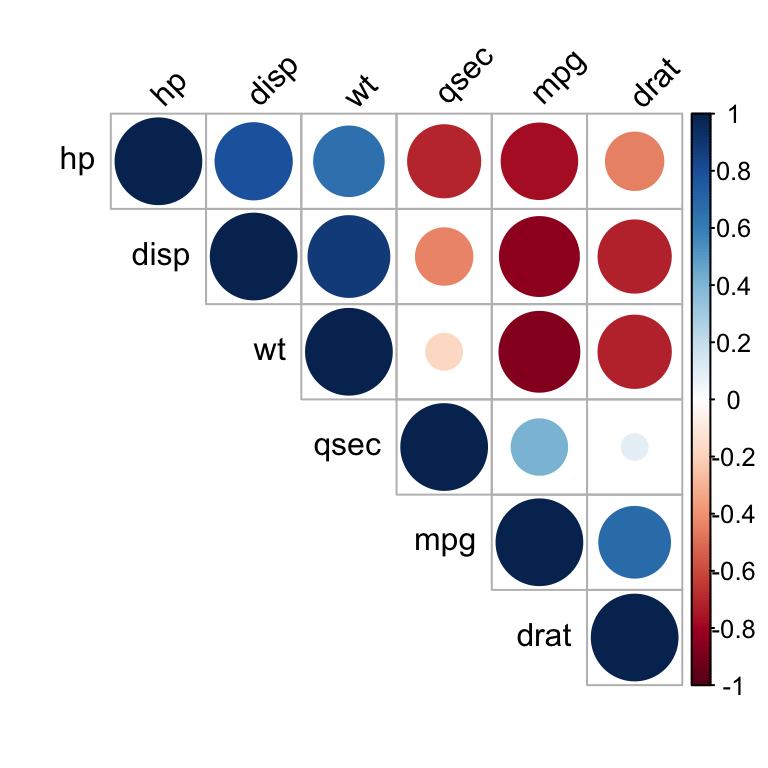
Correlation matrix - R software and statistics
Positive correlations are displayed in blue and negative correlations in red color. Color intensity and the size of the circle are proportional to the correlation coefficients. In the right side of the correlogram, the legend color shows the correlation coefficients and the corresponding colors.
- The correlation matrix is reordered according to the correlation coefficient using “hclust” method.
- tl.col (for text label color) and tl.srt (for text label string rotation) are used to change text colors and rotations.
- Possible values for the argument type are : “upper”, “lower”, “full”
Read more : visualize a correlation matrix using corrplot.
It’s also possible to combine correlogram with the significance test. We’ll use the result res.cor2 generated in the previous section with rcorr() function [in Hmisc package]:
# Insignificant correlation are crossed
corrplot(res2$r, type="upper", order="hclust",
         p.mat = res2$P, sig.level = 0.01, insig = "blank")
# Insignificant correlations are leaved blank
corrplot(res2$r, type="upper", order="hclust",
         p.mat = res2$P, sig.level = 0.01, insig = "blank")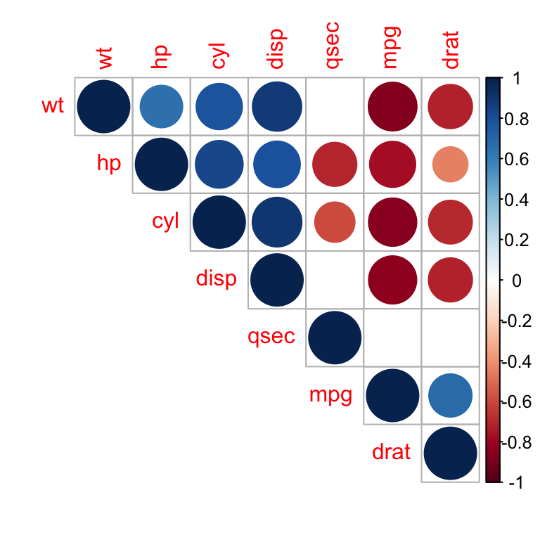
Correlation matrix - R software and statistics
In the above plot, correlations with p-value > 0.01 are considered as insignificant. In this case the correlation coefficient values are leaved blank or crosses are added.
Use chart.Correlation(): Draw scatter plots
The function chart.Correlation()[ in the package PerformanceAnalytics], can be used to display a chart of a correlation matrix.
- Install PerformanceAnalytics:
install.packages("PerformanceAnalytics")- Use chart.Correlation():
library("PerformanceAnalytics")
my_data <- mtcars[, c(1,3,4,5,6,7)]
chart.Correlation(my_data, histogram=TRUE, pch=19)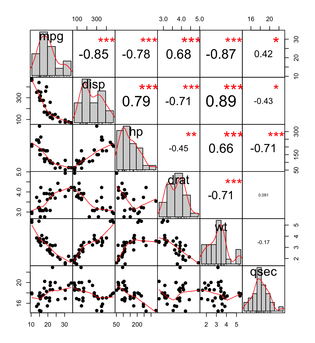
scatter plot, chart
In the above plot:
- The distribution of each variable is shown on the diagonal.
- On the bottom of the diagonal : the bivariate scatter plots with a fitted line are displayed
- On the top of the diagonal : the value of the correlation plus the significance level as stars
- Each significance level is associated to a symbol : p-values(0, 0.001, 0.01, 0.05, 0.1, 1) <=> symbols(“***”, “**”, “*”, “.”, " “)
Use heatmap()
# Get some colors
col<- colorRampPalette(c("blue", "white", "red"))(20)
heatmap(x = res, col = col, symm = TRUE)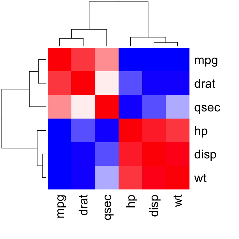
Heatmap of correlation matrix
- x : the correlation matrix to be plotted
- col : color palettes
- symm : logical indicating if x should be treated symmetrically; can only be true when x is a square matrix.
Online software to analyze and visualize a correlation matrix

Take me to the correlation matrix calculator
The software can be used as follow :
- Go to the web application : correlation matrix calculator
- Upload a .txt tab or a CSV file containing your data (columns are variables). The supported file formats are described here. You can use the demo data available on the calculator web page by clicking on the corresponding link.
- After uploading, an overview of a part of your file is shown to check that the data are correctly imported. If the data are not correctly displayed, please make sure that the format of your file is OK here.
- Click on the ‘Analyze’ button and select at least 2 variables to calculate the correlation matrix. By default, all variables are selected. Please, deselect the columns containing texts. You can also select the correlation methods (Pearson, Spearman or Kendall). Default is the Pearson method.
- Click the OK button
- Results : the output of the software includes :
- The correlation matrix
- The visualization of the correlation matrix as a correlogram
- A web link to export the results as .txt tab file
Note that, you can specify the alternative hypothesis to use for the correlation test by clicking on the button “Advanced options”.
Choose one of the 3 options :
- Two-sided
- Correlation < 0 for “less”
- Correlation > 0 for “greater”
Summarry
- Use cor() function for simple correlation analysis
- Use rcorr() function from Hmisc package to compute matrix of correlation coefficients and matrix of p-values in single step.
- Use symnum(), corrplot()[from corrplot package], chart.Correlation() [from PerformanceAnalytics package], or heatmap() functions to visualize a correlation matrix.
Infos
This analysis has been performed using R software (ver. 3.2.4).
Show me some love with the like buttons below... Thank you and please don't forget to share and comment below!!
Montrez-moi un peu d'amour avec les like ci-dessous ... Merci et n'oubliez pas, s'il vous plaît, de partager et de commenter ci-dessous!
Recommended for You!


Recommended for you
This section contains the best data science and self-development resources to help you on your path.
Books - Data Science
Our Books
- Practical Guide to Cluster Analysis in R by A. Kassambara (Datanovia)
- Practical Guide To Principal Component Methods in R by A. Kassambara (Datanovia)
- Machine Learning Essentials: Practical Guide in R by A. Kassambara (Datanovia)
- R Graphics Essentials for Great Data Visualization by A. Kassambara (Datanovia)
- GGPlot2 Essentials for Great Data Visualization in R by A. Kassambara (Datanovia)
- Network Analysis and Visualization in R by A. Kassambara (Datanovia)
- Practical Statistics in R for Comparing Groups: Numerical Variables by A. Kassambara (Datanovia)
- Inter-Rater Reliability Essentials: Practical Guide in R by A. Kassambara (Datanovia)
Others
- R for Data Science: Import, Tidy, Transform, Visualize, and Model Data by Hadley Wickham & Garrett Grolemund
- Hands-On Machine Learning with Scikit-Learn, Keras, and TensorFlow: Concepts, Tools, and Techniques to Build Intelligent Systems by Aurelien Géron
- Practical Statistics for Data Scientists: 50 Essential Concepts by Peter Bruce & Andrew Bruce
- Hands-On Programming with R: Write Your Own Functions And Simulations by Garrett Grolemund & Hadley Wickham
- An Introduction to Statistical Learning: with Applications in R by Gareth James et al.
- Deep Learning with R by François Chollet & J.J. Allaire
- Deep Learning with Python by François Chollet
Click to follow us on Facebook :
Comment this article by clicking on "Discussion" button (top-right position of this page)