Agilent data

Download raw data

The raw data files for this lab are in the rawdata repository, available here:
https://github.com/genomicsclass/rawdata.
Click Download ZIP in order to download all the files, unzip this file which should result in a rawdata-master folder. Rename this folder to rawdata.

Read Agilent data

Agilent data is a two color arrays. For two-color arrays it’s slightly more complicated, because you have a pairing of files (red and green channels). Different scanners spit out different formats for this. So the target information will be a little bit different. limma package is used to read the files. The readTargets function tells you what’s in the red and the green channels.

The function read.maimages(microarray images) is used to read the data. You have to tell it what software produced the images. There’s different software for that, although these days, there’s a default that works pretty broadly. So all we’re doing now is telling it where the files are. We tell it what imaging software was used to produce these files (“genepix”). The function read.maimages, stores red and green separately.

library(limma)
library(rafalib)#installed from github
#Define a base directory
basedir <- "~/hubiC/Documents/R/doc/english/genomics/rawdata/agilent"
setwd(basedir)
#Read sample information table : it tells you what's in the red channel and the green channel
targets <- readTargets("TargetBeta7.txt")
#Read microarray files : Red and green are stored separately
RG <- read.maimages(targets$FileName, source="genepix")

## Read 6Hs.195.1.gpr 
## Read 6Hs.168.gpr 
## Read 6Hs.166.gpr 
## Read 6Hs.187.1.gpr 
## Read 6Hs.194.gpr 
## Read 6Hs.243.1.gpr

Normalization

Data are normalized using MA.RG function. It stores the information as the log ratio– that’s the M– and the average of the logs, which is the A.

#Normalization
MA <- MA.RG(RG,bc.method="none")

MA plot

Just to give you a quick idea of what you can do with this. You can do an MA plot. You just plot the A versus the M.

#Normalization
MA <- MA.RG(RG,bc.method="none")
#MA plot
plot(MA$A[,1],MA$M[,1])#MA plot for the first sample

Array image

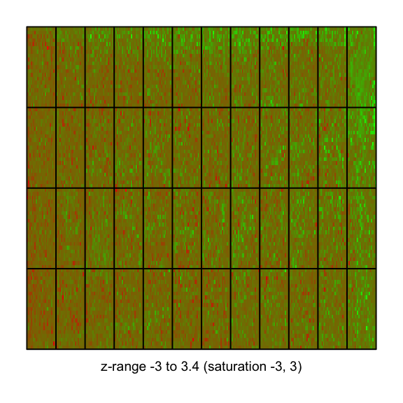
Another nice feature is to make images pretty quickly.

#Array image
imageplot(MA$M[,2], RG$printer, zlim=c(-3,3))

This is a nice example where we see an image where there seems to be a little bit of a problem. If you look at the edge, you see that it's quite green, compared to the middle, which is redder. Then you have too much red on the left. So we're detecting that there's somewhat of a problem in this file.

Licence

Licence

References

https://github.com/genomicsclass

Recommended for you