


Simple Linear Regression in R
The simple linear regression is used to predict a quantitative outcome y on the basis of one single predictor variable x. The goal is to build a mathematical model (or formula) that defines y as a function of the x variable.
Once, we built a statistically significant model, it’s possible to use it for predicting future outcome on the basis of new x values.
Consider that, we want to evaluate the impact of advertising budgets of three medias (youtube, facebook and newspaper) on future sales. This example of problem can be modeled with linear regression.
Contents:

Formula and basics
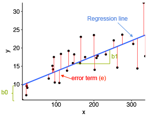
The mathematical formula of the linear regression can be written as y = b0 + b1*x + e, where:
b0andb1are known as the regression beta coefficients or parameters:b0is the intercept of the regression line; that is the predicted value whenx = 0.b1is the slope of the regression line.
eis the error term (also known as the residual errors), the part of y that can be explained by the regression model
The figure below illustrates the linear regression model, where:
- the best-fit regression line is in blue
- the intercept (b0) and the slope (b1) are shown in green
- the error terms (e) are represented by vertical red lines
From the scatter plot above, it can be seen that not all the data points fall exactly on the fitted regression line. Some of the points are above the blue curve and some are below it; overall, the residual errors (e) have approximately mean zero.
The sum of the squares of the residual errors are called the Residual Sum of Squares or RSS.
The average variation of points around the fitted regression line is called the Residual Standard Error (RSE). This is one the metrics used to evaluate the overall quality of the fitted regression model. The lower the RSE, the better it is.
Since the mean error term is zero, the outcome variable y can be approximately estimated as follow:
y ~ b0 + b1*x
Mathematically, the beta coefficients (b0 and b1) are determined so that the RSS is as minimal as possible. This method of determining the beta coefficients is technically called least squares regression or ordinary least squares (OLS) regression.
Once, the beta coefficients are calculated, a t-test is performed to check whether or not these coefficients are significantly different from zero. A non-zero beta coefficients means that there is a significant relationship between the predictors (x) and the outcome variable (y).
Loading required R packages
Load required packages:
tidyversefor data manipulation and visualizationggpubr: creates easily a publication ready-plot
library(tidyverse)
library(ggpubr)
theme_set(theme_pubr())
Examples of data and problem
We’ll use the marketing data set [datarium package]. It contains the impact of three advertising medias (youtube, facebook and newspaper) on sales. Data are the advertising budget in thousands of dollars along with the sales. The advertising experiment has been repeated 200 times with different budgets and the observed sales have been recorded.
First install the datarium package using devtools::install_github("kassmbara/datarium"), then load and inspect the marketing data as follow:
Inspect the data:
# Load the package
data("marketing", package = "datarium")
head(marketing, 4)
## youtube facebook newspaper sales
## 1 276.1 45.4 83.0 26.5
## 2 53.4 47.2 54.1 12.5
## 3 20.6 55.1 83.2 11.2
## 4 181.8 49.6 70.2 22.2We want to predict future sales on the basis of advertising budget spent on youtube.
Visualization
- Create a scatter plot displaying the sales units versus youtube advertising budget.
- Add a smoothed line
ggplot(marketing, aes(x = youtube, y = sales)) +
  geom_point() +
  stat_smooth()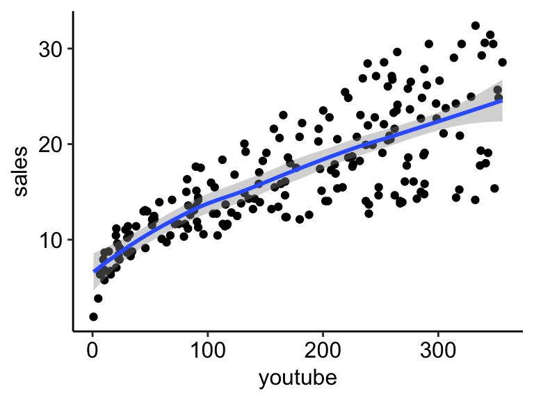
The graph above suggests a linearly increasing relationship between the sales and the youtube variables. This is a good thing, because, one important assumption of the linear regression is that the relationship between the outcome and predictor variables is linear and additive.
It’s also possible to compute the correlation coefficient between the two variables using the R function cor():
cor(marketing$sales, marketing$youtube)## [1] 0.782The correlation coefficient measures the level of the association between two variables x and y. Its value ranges between -1 (perfect negative correlation: when x increases, y decreases) and +1 (perfect positive correlation: when x increases, y increases).
A value closer to 0 suggests a weak relationship between the variables. A low correlation (-0.2 < x < 0.2) probably suggests that much of variation of the outcome variable (y) is not explained by the predictor (x). In such case, we should probably look for better predictor variables.
In our example, the correlation coefficient is large enough, so we can continue by building a linear model of y as a function of x.
Computation
The simple linear regression tries to find the best line to predict sales on the basis of youtube advertising budget.
The linear model equation can be written as follow: sales = b0 + b1 * youtube
The R function lm() can be used to determine the beta coefficients of the linear model:
model <- lm(sales ~ youtube, data = marketing)
model
##
## Call:
## lm(formula = sales ~ youtube, data = marketing)
##
## Coefficients:
## (Intercept) youtube
## 8.4391 0.0475The results show the intercept and the beta coefficient for the youtube variable.
Interpretation
From the output above:
the estimated regression line equation can be written as follow:
sales = 8.44 + 0.048*youtubethe intercept (
b0) is 8.44. It can be interpreted as the predicted sales unit for a zero youtube advertising budget. Recall that, we are operating in units of thousand dollars. This means that, for a youtube advertising budget equal zero, we can expect a sale of 8.44 *1000 = 8440 dollars.the regression beta coefficient for the variable youtube (
b1), also known as the slope, is 0.048. This means that, for a youtube advertising budget equal to 1000 dollars, we can expect an increase of 48 units (0.048*1000) in sales. That is,sales = 8.44 + 0.048*1000 = 56.44 units. As we are operating in units of thousand dollars, this represents a sale of 56440 dollars.
Regression line
To add the regression line onto the scatter plot, you can use the function stat_smooth() [ggplot2]. By default, the fitted line is presented with confidence interval around it. The confidence bands reflect the uncertainty about the line. If you don’t want to display it, specify the option se = FALSE in the function stat_smooth().
ggplot(marketing, aes(youtube, sales)) +
  geom_point() +
  stat_smooth(method = lm)
Model assessment
In the previous section, we built a linear model of sales as a function of youtube advertising budget: sales = 8.44 + 0.048*youtube.
Before using this formula to predict future sales, you should make sure that this model is statistically significant, that is:
- there is a statistically significant relationship between the predictor and the outcome variables
- the model that we built fits very well the data in our hand.
In this section, we’ll describe how to check the quality of a linear regression model.
Model summary
We start by displaying the statistical summary of the model using the R function summary():
summary(model)##
## Call:
## lm(formula = sales ~ youtube, data = marketing)
##
## Residuals:
## Min 1Q Median 3Q Max
## -10.06 -2.35 -0.23 2.48 8.65
##
## Coefficients:
## Estimate Std. Error t value Pr(>|t|)
## (Intercept) 8.43911 0.54941 15.4 <2e-16 ***
## youtube 0.04754 0.00269 17.7 <2e-16 ***
## ---
## Signif. codes: 0 '***' 0.001 '**' 0.01 '*' 0.05 '.' 0.1 ' ' 1
##
## Residual standard error: 3.91 on 198 degrees of freedom
## Multiple R-squared: 0.612, Adjusted R-squared: 0.61
## F-statistic: 312 on 1 and 198 DF, p-value: <2e-16The summary outputs shows 6 components, including:
- Call. Shows the function call used to compute the regression model.
- Residuals. Provide a quick view of the distribution of the residuals, which by definition have a mean zero. Therefore, the median should not be far from zero, and the minimum and maximum should be roughly equal in absolute value.
- Coefficients. Shows the regression beta coefficients and their statistical significance. Predictor variables, that are significantly associated to the outcome variable, are marked by stars.
- Residual standard error (RSE), R-squared (R2) and the F-statistic are metrics that are used to check how well the model fits to our data.
Coefficients significance
The coefficients table, in the model statistical summary, shows:
- the estimates of the beta coefficients
- the standard errors (SE), which defines the accuracy of beta coefficients. For a given beta coefficient, the SE reflects how the coefficient varies under repeated sampling. It can be used to compute the confidence intervals and the t-statistic.
- the t-statistic and the associated p-value, which defines the statistical significance of the beta coefficients.
##             Estimate Std. Error t value Pr(>|t|)
## (Intercept)   8.4391    0.54941    15.4 1.41e-35
## youtube       0.0475    0.00269    17.7 1.47e-42
t-statistic and p-values:
For a given predictor, the t-statistic (and its associated p-value) tests whether or not there is a statistically significant relationship between a given predictor and the outcome variable, that is whether or not the beta coefficient of the predictor is significantly different from zero.
The statistical hypotheses are as follow:
- Null hypothesis (H0): the coefficients are equal to zero (i.e., no relationship between x and y)
- Alternative Hypothesis (Ha): the coefficients are not equal to zero (i.e., there is some relationship between x and y)
Mathematically, for a given beta coefficient (b), the t-test is computed as t = (b - 0)/SE(b), where SE(b) is the standard error of the coefficient b. The t-statistic measures the number of standard deviations that b is away from 0. Thus a large t-statistic will produce a small p-value.
The higher the t-statistic (and the lower the p-value), the more significant the predictor. The symbols to the right visually specifies the level of significance. The line below the table shows the definition of these symbols; one star means 0.01 < p < 0.05. The more the stars beside the variable’s p-value, the more significant the variable.
A statistically significant coefficient indicates that there is an association between the predictor (x) and the outcome (y) variable.
In our example, both the p-values for the intercept and the predictor variable are highly significant, so we can reject the null hypothesis and accept the alternative hypothesis, which means that there is a significant association between the predictor and the outcome variables.
The t-statistic is a very useful guide for whether or not to include a predictor in a model. High t-statistics (which go with low p-values near 0) indicate that a predictor should be retained in a model, while very low t-statistics indicate a predictor could be dropped (P. Bruce and Bruce 2017).
Standard errors and confidence intervals:
The standard error measures the variability/accuracy of the beta coefficients. It can be used to compute the confidence intervals of the coefficients.
For example, the 95% confidence interval for the coefficient b1 is defined as b1 +/- 2*SE(b1), where:
- the lower limits of b1 =
b1 - 2*SE(b1) = 0.047 - 2*0.00269 = 0.042 - the upper limits of b1 =
b1 + 2*SE(b1) = 0.047 + 2*0.00269 = 0.052
That is, there is approximately a 95% chance that the interval [0.042, 0.052] will contain the true value of b1. Similarly the 95% confidence interval for b0 can be computed as b0 +/- 2*SE(b0).
To get these information, simply type:
confint(model)## 2.5 % 97.5 %
## (Intercept) 7.3557 9.5226
## youtube 0.0422 0.0528Model accuracy
Once you identified that, at least, one predictor variable is significantly associated the outcome, you should continue the diagnostic by checking how well the model fits the data. This process is also referred to as the goodness-of-fit
The overall quality of the linear regression fit can be assessed using the following three quantities, displayed in the model summary:
- The Residual Standard Error (RSE).
- The R-squared (R2)
- F-statistic
##    rse r.squared f.statistic  p.value
## 1 3.91 0.612 312 1.47e-42- Residual standard error (RSE).
The RSE (also known as the model sigma) is the residual variation, representing the average variation of the observations points around the fitted regression line. This is the standard deviation of residual errors.
RSE provides an absolute measure of patterns in the data that can’t be explained by the model. When comparing two models, the model with the small RSE is a good indication that this model fits the best the data.
Dividing the RSE by the average value of the outcome variable will give you the prediction error rate, which should be as small as possible.
In our example, RSE = 3.91, meaning that the observed sales values deviate from the true regression line by approximately 3.9 units in average.
Whether or not an RSE of 3.9 units is an acceptable prediction error is subjective and depends on the problem context. However, we can calculate the percentage error. In our data set, the mean value of sales is 16.827, and so the percentage error is 3.9/16.827 = 23%.
sigma(model)*100/mean(marketing$sales)## [1] 23.2- R-squared and Adjusted R-squared:
The R-squared (R2) ranges from 0 to 1 and represents the proportion of information (i.e. variation) in the data that can be explained by the model. The adjusted R-squared adjusts for the degrees of freedom.
The R2 measures, how well the model fits the data. For a simple linear regression, R2 is the square of the Pearson correlation coefficient.
A high value of R2 is a good indication. However, as the value of R2 tends to increase when more predictors are added in the model, such as in multiple linear regression model, you should mainly consider the adjusted R-squared, which is a penalized R2 for a higher number of predictors.
- An (adjusted) R2 that is close to 1 indicates that a large proportion of the variability in the outcome has been explained by the regression model.
- A number near 0 indicates that the regression model did not explain much of the variability in the outcome.
- F-Statistic:
The F-statistic gives the overall significance of the model. It assess whether at least one predictor variable has a non-zero coefficient.
In a simple linear regression, this test is not really interesting since it just duplicates the information in given by the t-test, available in the coefficient table. In fact, the F test is identical to the square of the t test: 312.1 = (17.67)^2. This is true in any model with 1 degree of freedom.
The F-statistic becomes more important once we start using multiple predictors as in multiple linear regression.
A large F-statistic will corresponds to a statistically significant p-value (p < 0.05). In our example, the F-statistic equal 312.14 producing a p-value of 1.46e-42, which is highly significant.
Summary
After computing a regression model, a first step is to check whether, at least, one predictor is significantly associated with outcome variables.
If one or more predictors are significant, the second step is to assess how well the model fits the data by inspecting the Residuals Standard Error (RSE), the R2 value and the F-statistics. These metrics give the overall quality of the model.
- RSE: Closer to zero the better
- R-Squared: Higher the better
- F-statistic: Higher the better
Read more
- Introduction to statistical learning (James et al. 2014)
- Practical Statistics for Data Scientists (P. Bruce and Bruce 2017)
References
Bruce, Peter, and Andrew Bruce. 2017. Practical Statistics for Data Scientists. O’Reilly Media.
James, Gareth, Daniela Witten, Trevor Hastie, and Robert Tibshirani. 2014. An Introduction to Statistical Learning: With Applications in R. Springer Publishing Company, Incorporated.