Articles - Classification Methods Essentials

Loading required R packages

• tidyverse for easy data manipulation and visualization
• caret for easy machine learning workflow

library(tidyverse)
library(caret)
theme_set(theme_classic())

Preparing the data

We’ll use the iris data set, introduced in Chapter @ref(classification-in-r), for predicting iris species based on the predictor variables Sepal.Length, Sepal.Width, Petal.Length, Petal.Width.

Discriminant analysis can be affected by the scale/unit in which predictor variables are measured. It’s generally recommended to standardize/normalize continuous predictor before the analysis.

1. Split the data into training and test set:

# Load the data
data("iris")
# Split the data into training (80%) and test set (20%)
set.seed(123)
training.samples <- iris$Species %>%
  createDataPartition(p = 0.8, list = FALSE)
train.data <- iris[training.samples, ]
test.data <- iris[-training.samples, ]

2. Normalize the data. Categorical variables are automatically ignored.

# Estimate preprocessing parameters
preproc.param <- train.data %>% 
  preProcess(method = c("center", "scale"))
# Transform the data using the estimated parameters
train.transformed <- preproc.param %>% predict(train.data)
test.transformed <- preproc.param %>% predict(test.data)

Linear discriminant analysis - LDA

The LDA algorithm starts by finding directions that maximize the separation between classes, then use these directions to predict the class of individuals. These directions, called linear discriminants, are a linear combinations of predictor variables.

LDA assumes that predictors are normally distributed (Gaussian distribution) and that the different classes have class-specific means and equal variance/covariance.

Before performing LDA, consider:

• Inspecting the univariate distributions of each variable and make sure that they are normally distribute. If not, you can transform them using log and root for exponential distributions and Box-Cox for skewed distributions.
• removing outliers from your data and standardize the variables to make their scale comparable.

The linear discriminant analysis can be easily computed using the function lda() [MASS package].

Quick start R code:

library(MASS)
# Fit the model
model <- lda(Species~., data = train.transformed)
# Make predictions
predictions <- model %>% predict(test.transformed)
# Model accuracy
mean(predictions$class==test.transformed$Species)

Compute LDA:

library(MASS)
model <- lda(Species~., data = train.transformed)
model

## Call:
## lda(Species ~ ., data = train.transformed)
## 
## Prior probabilities of groups:
##     setosa versicolor  virginica 
##      0.333      0.333      0.333 
## 
## Group means:
##            Sepal.Length Sepal.Width Petal.Length Petal.Width
## setosa           -1.012       0.787       -1.293      -1.250
## versicolor        0.117      -0.648        0.272       0.154
## virginica         0.895      -0.139        1.020       1.095
## 
## Coefficients of linear discriminants:
##                 LD1     LD2
## Sepal.Length  0.911  0.0318
## Sepal.Width   0.648  0.8985
## Petal.Length -4.082 -2.2272
## Petal.Width  -2.313  2.6544
## 
## Proportion of trace:
##    LD1    LD2 
## 0.9905 0.0095

LDA determines group means and computes, for each individual, the probability of belonging to the different groups. The individual is then affected to the group with the highest probability score.

The lda() outputs contain the following elements:

• Prior probabilities of groups: the proportion of training observations in each group. For example, there are 31% of the training observations in the setosa group
• Group means: group center of gravity. Shows the mean of each variable in each group.
• Coefficients of linear discriminants: Shows the linear combination of predictor variables that are used to form the LDA decision rule. for example, LD1 = 0.91*Sepal.Length + 0.64*Sepal.Width - 4.08*Petal.Length - 2.3*Petal.Width. Similarly, LD2 = 0.03*Sepal.Length + 0.89*Sepal.Width - 2.2*Petal.Length - 2.6*Petal.Width.

Using the function plot() produces plots of the linear discriminants, obtained by computing LD1 and LD2 for each of the training observations.

plot(model)

Make predictions:

predictions <- model %>% predict(test.transformed)
names(predictions)

## [1] "class"     "posterior" "x"

The predict() function returns the following elements:

• class: predicted classes of observations.
• posterior: is a matrix whose columns are the groups, rows are the individuals and values are the posterior probability that the corresponding observation belongs to the groups.
• x: contains the linear discriminants, described above

Inspect the results:

# Predicted classes
head(predictions$class, 6)
# Predicted probabilities of class memebership.
head(predictions$posterior, 6) 
# Linear discriminants
head(predictions$x, 3) 

Note that, you can create the LDA plot using ggplot2 as follow:

lda.data <- cbind(train.transformed, predict(model)$x)
ggplot(lda.data, aes(LD1, LD2)) +
  geom_point(aes(color = Species))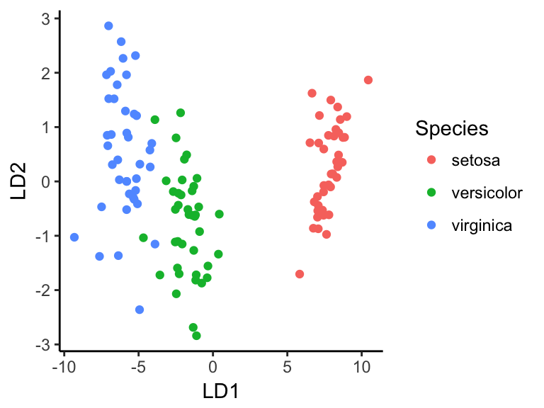

Model accuracy:

You can compute the model accuracy as follow:

mean(predictions$class==test.transformed$Species)

## [1] 1

Note that, by default, the probability cutoff used to decide group-membership is 0.5 (random guessing). For example, the number of observations in the setosa group can be re-calculated using:

sum(predictions$posterior[ ,1] >=.5)

## [1] 10

In some situations, you might want to increase the precision of the model. In this case you can fine-tune the model by adjusting the posterior probability cutoff. For example, you can increase or lower the cutoff.

Variable selection:

Note that, if the predictor variables are standardized before computing LDA, the discriminator weights can be used as measures of variable importance for feature selection.

Quadratic discriminant analysis - QDA

QDA is little bit more flexible than LDA, in the sense that it does not assumes the equality of variance/covariance. In other words, for QDA the covariance matrix can be different for each class.

LDA tends to be a better than QDA when you have a small training set.

In contrast, QDA is recommended if the training set is very large, so that the variance of the classifier is not a major issue, or if the assumption of a common covariance matrix for the K classes is clearly untenable (James et al. 2014).

QDA can be computed using the R function qda() [MASS package]

library(MASS)
# Fit the model
model <- qda(Species~., data = train.transformed)
model
# Make predictions
predictions <- model %>% predict(test.transformed)
# Model accuracy
mean(predictions$class == test.transformed$Species)

Mixture discriminant analysis - MDA

The LDA classifier assumes that each class comes from a single normal (or Gaussian) distribution. This is too restrictive.

For MDA, there are classes, and each class is assumed to be a Gaussian mixture of subclasses, where each data point has a probability of belonging to each class. Equality of covariance matrix, among classes, is still assumed.

library(mda)
# Fit the model
model <- mda(Species~., data = train.transformed)
model
# Make predictions
predicted.classes <- model %>% predict(test.transformed)
# Model accuracy
mean(predicted.classes == test.transformed$Species)

MDA might outperform LDA and QDA is some situations, as illustrated below. In this example data, we have 3 main groups of individuals, each having 3 no adjacent subgroups. The solid black lines on the plot represent the decision boundaries of LDA, QDA and MDA. It can be seen that the MDA classifier have identified correctly the subclasses compared to LDA and QDA, which were not good at all in modeling this data.

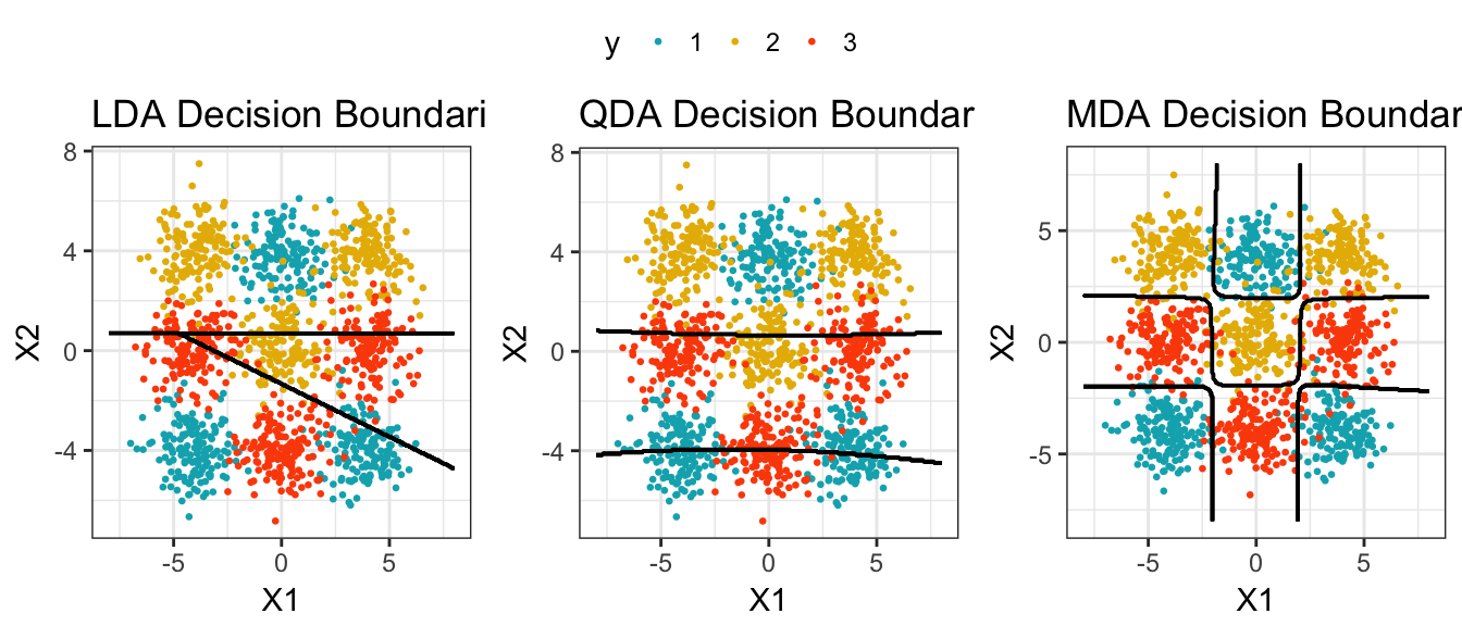
The code for generating the above plots is from John Ramey

Flexible discriminant analysis - FDA

FDA is a flexible extension of LDA that uses non-linear combinations of predictors such as splines. FDA is useful to model multivariate non-normality or non-linear relationships among variables within each group, allowing for a more accurate classification.

library(mda)
# Fit the model
model <- fda(Species~., data = train.transformed)
# Make predictions
predicted.classes <- model %>% predict(test.transformed)
# Model accuracy
mean(predicted.classes == test.transformed$Species)

Regularized discriminant analysis

RDA builds a classification rule by regularizing the group covariance matrices (Friedman 1989) allowing a more robust model against multicollinearity in the data. This might be very useful for a large multivariate data set containing highly correlated predictors.

Regularized discriminant analysis is a kind of a trade-off between LDA and QDA. Recall that, in LDA we assume equality of covariance matrix for all of the classes. QDA assumes different covariance matrices for all the classes. Regularized discriminant analysis is an intermediate between LDA and QDA.

RDA shrinks the separate covariances of QDA toward a common covariance as in LDA. This improves the estimate of the covariance matrices in situations where the number of predictors is larger than the number of samples in the training data, potentially leading to an improvement of the model accuracy.

library(klaR)
# Fit the model
model <- rda(Species~., data = train.transformed)
# Make predictions
predictions <- model %>% predict(test.transformed)
# Model accuracy
mean(predictions$class == test.transformed$Species)

Discussion

We have described linear discriminant analysis (LDA) and extensions for predicting the class of an observations based on multiple predictor variables. Discriminant analysis is more suitable to multiclass classification problems compared to the logistic regression (Chapter @ref(logistic-regression)).

LDA assumes that the different classes has the same variance or covariance matrix. We have described many extensions of LDA in this chapter. The most popular extension of LDA is the quadratic discriminant analysis (QDA), which is more flexible than LDA in the sens that it does not assume the equality of group covariance matrices.

LDA tends to be better than QDA for small data set. QDA is recommended for large training data set.

References

Friedman, Jerome H. 1989. “Regularized Discriminant Analysis.” Journal of the American Statistical Association 84 (405). Taylor & Francis: 165–75. doi:10.1080/01621459.1989.10478752.
James, Gareth, Daniela Witten, Trevor Hastie, and Robert Tibshirani. 2014. An Introduction to Statistical Learning: With Applications in R. Springer Publishing Company, Incorporated.