PCA in R Using Ade4: Quick Scripts
This article provides quick start R codes to compute principal component analysis (PCA) using the function dudi.pca() in the ade4 R package. We’ll use the factoextra R package to visualize the PCA results. We’ll describe also how to predict the coordinates for new individuals / variables data using ade4 functions.
Read more about the basics and the interpretation of principal component analysis in our previous article: PCA - Principal Component Analysis Essentials.

Contents:
Related Book:
Practical Guide to Principal Component Methods in R
Install and load packages
Install:
install.packages("magrittr")  # for piping %>%
install.packages("ade4")      # PCA computation
install.packages("factoextra")# PCA visualization
Load:
library(ade4)
library(factoextra)
library(magrittr)
Data sets
- Demo data:
decathlon2[in factoextra]. - Data description available at: PCA - Data format.
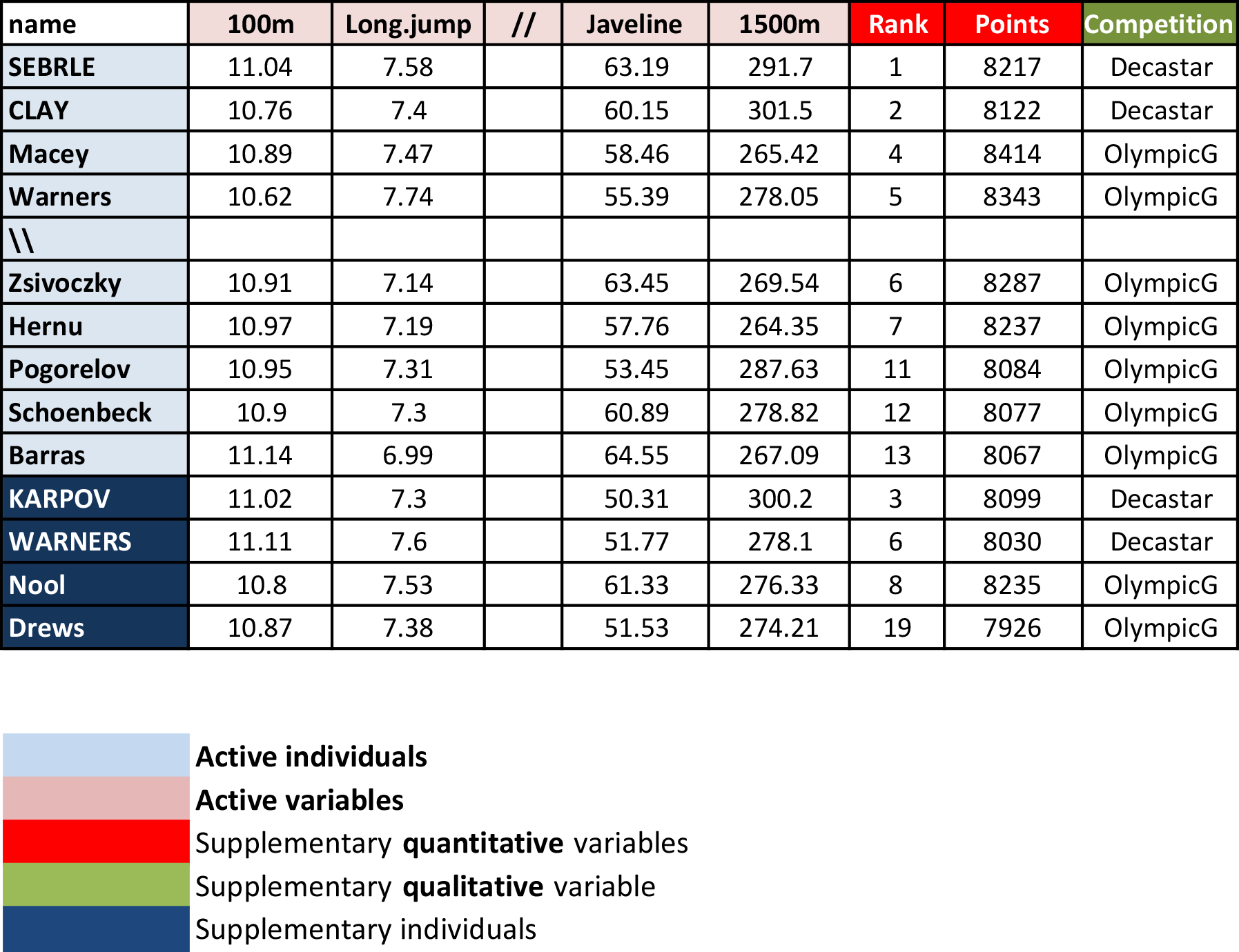
- Data contents:
- Active individuals (rows 1 to 23) and active variables (columns 1 to 10). Used to compute the PCA.
- Supplementary individuals (rows 24 to 27) and supplementary variables (columns 11 to 13). Their coordinates will be predicted using the PCA information and parameters obtained with active individuals/variables.
Load the data and extract only active individuals and variables:
library("factoextra")
data(decathlon2)
decathlon2.active <- decathlon2[1:23, 1:10]
head(decathlon2.active[, 1:6])
## X100m Long.jump Shot.put High.jump X400m X110m.hurdle
## SEBRLE 11.0 7.58 14.8 2.07 49.8 14.7
## CLAY 10.8 7.40 14.3 1.86 49.4 14.1
## BERNARD 11.0 7.23 14.2 1.92 48.9 15.0
## YURKOV 11.3 7.09 15.2 2.10 50.4 15.3
## ZSIVOCZKY 11.1 7.30 13.5 2.01 48.6 14.2
## McMULLEN 10.8 7.31 13.8 2.13 49.9 14.4Compute PCA using dudi.pca()
library(ade4)
res.pca <- dudi.pca(decathlon2.active,
                    scannf = FALSE,   # Hide scree plot
                    nf = 5            # Number of components kept in the results
                    )
Visualize PCA results
Visualize using factoextra
The factoextra R package creates ggplot2-based visualization.
- Visualize eigenvalues (scree plot). Show the percentage of variances explained by each principal component.
fviz_eig(res.pca)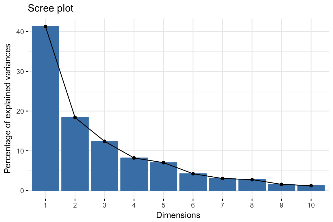
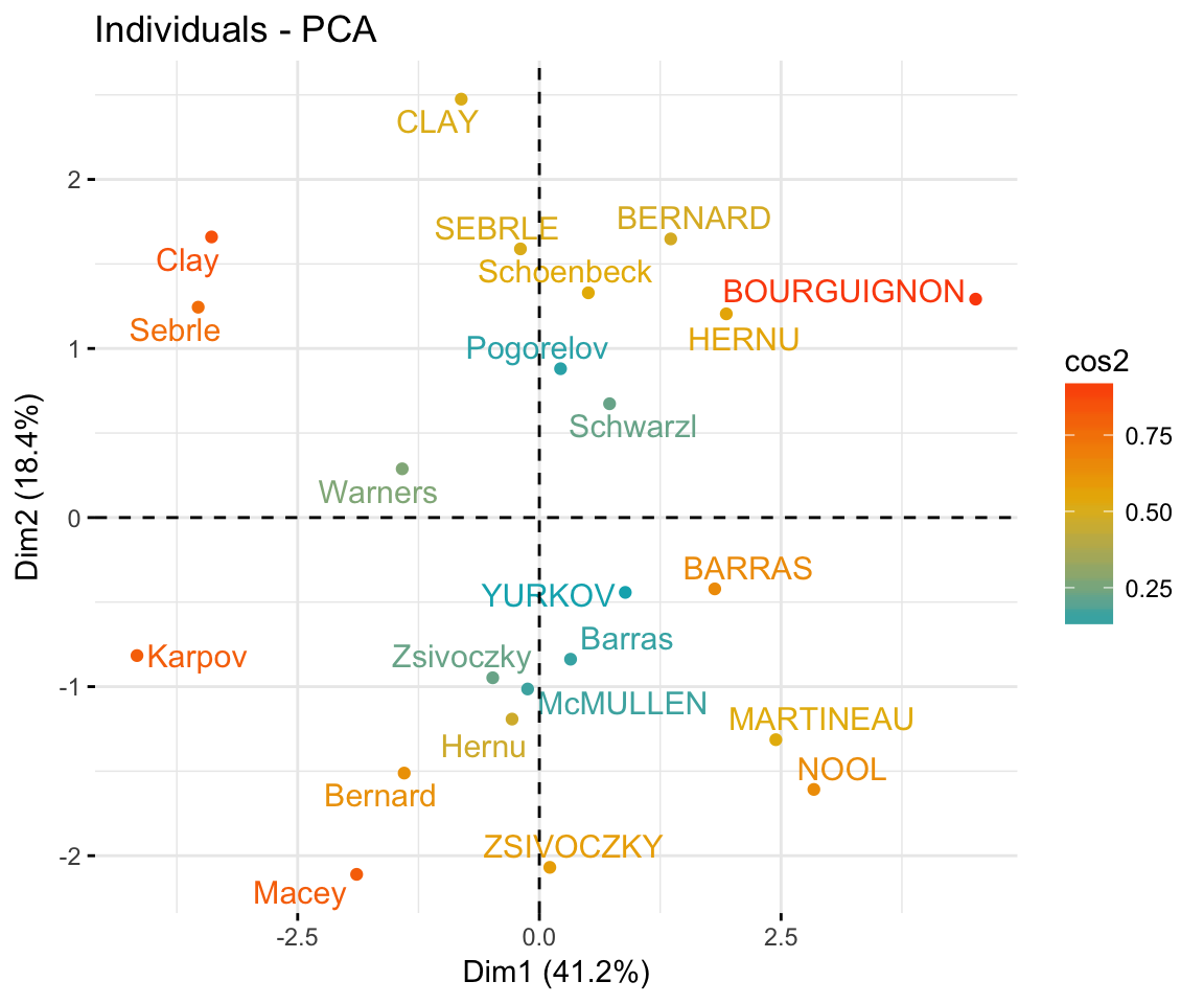
- Graph of individuals. Individuals with a similar profile are grouped together.
fviz_pca_ind(res.pca,
             col.ind = "cos2", # Color by the quality of representation
             gradient.cols = c("#00AFBB", "#E7B800", "#FC4E07"),
             repel = TRUE     # Avoid text overlapping
             )
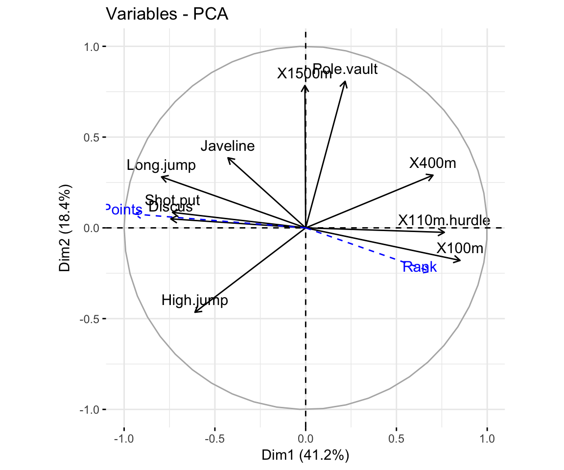
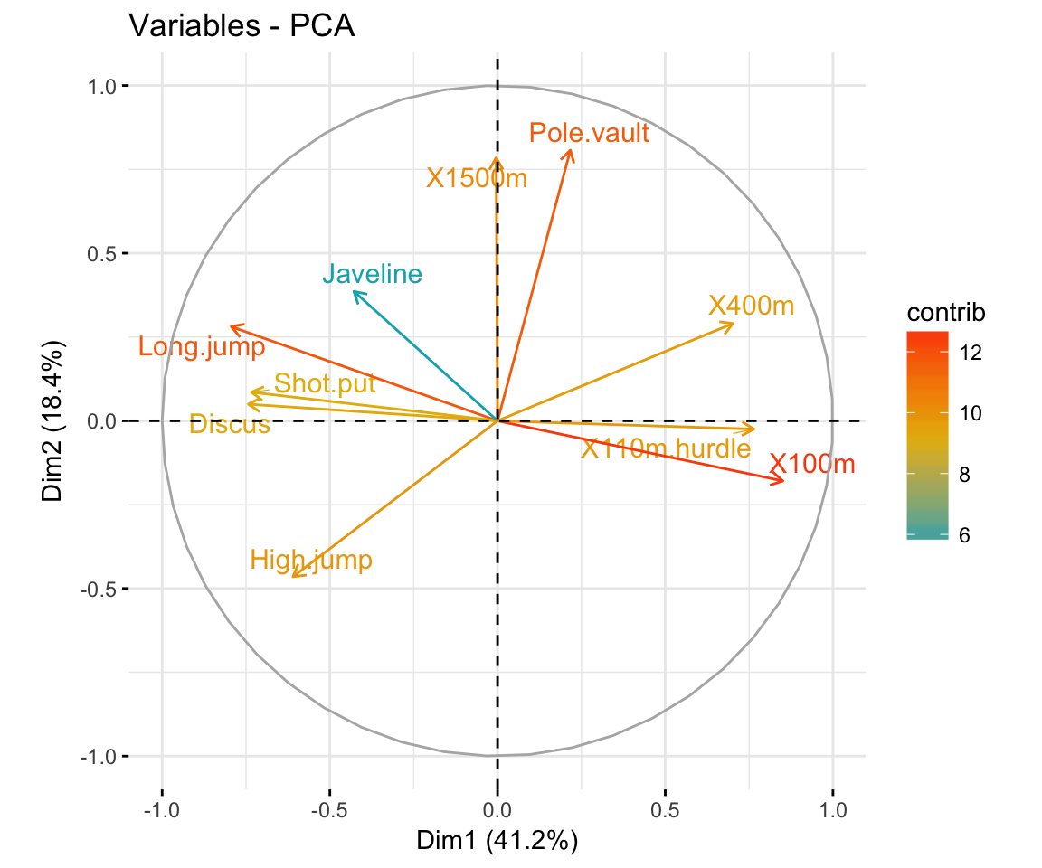
- Graph of variables. Positive correlated variables point to the same side of the plot. Negative correlated variables point to opposite sides of the graph.
fviz_pca_var(res.pca,
             col.var = "contrib", # Color by contributions to the PC
             gradient.cols = c("#00AFBB", "#E7B800", "#FC4E07"),
             repel = TRUE     # Avoid text overlapping
             )
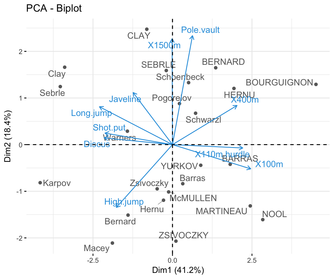
- Biplot of individuals and variables
fviz_pca_biplot(res.pca, repel = TRUE,
                col.var = "#2E9FDF", # Variables color
                col.ind = "#696969"  # Individuals color
                )
Visualize using ade4
The ade4 package creates R base plots.
# Scree plot
screeplot(res.pca, main = "Screeplot - Eigenvalues")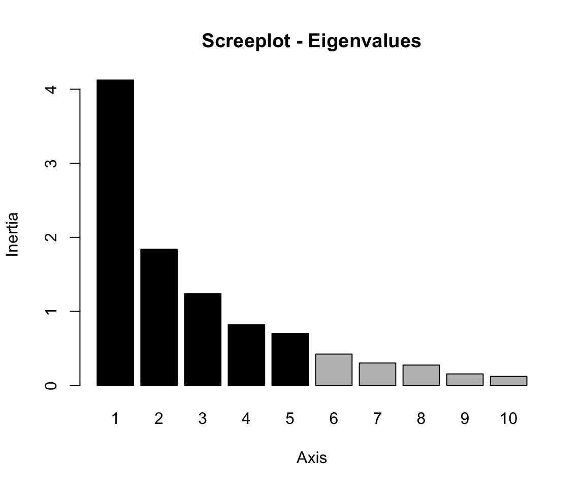
# Correlation circle of variables
s.corcircle(res.pca$co)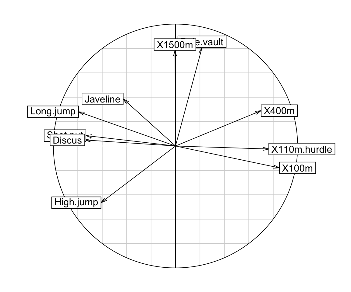
# Graph of individuals
s.label(res.pca$li,
        xax = 1,     # Dimension 1
        yax = 2)     # Dimension 2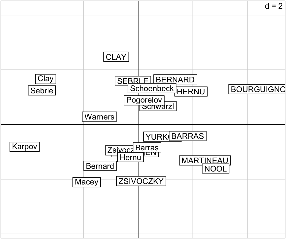
# Biplot of individuals and variables
scatter(res.pca,
        posieig = "none", # Hide the scree plot
        clab.row = 0      # Hide row labels
        )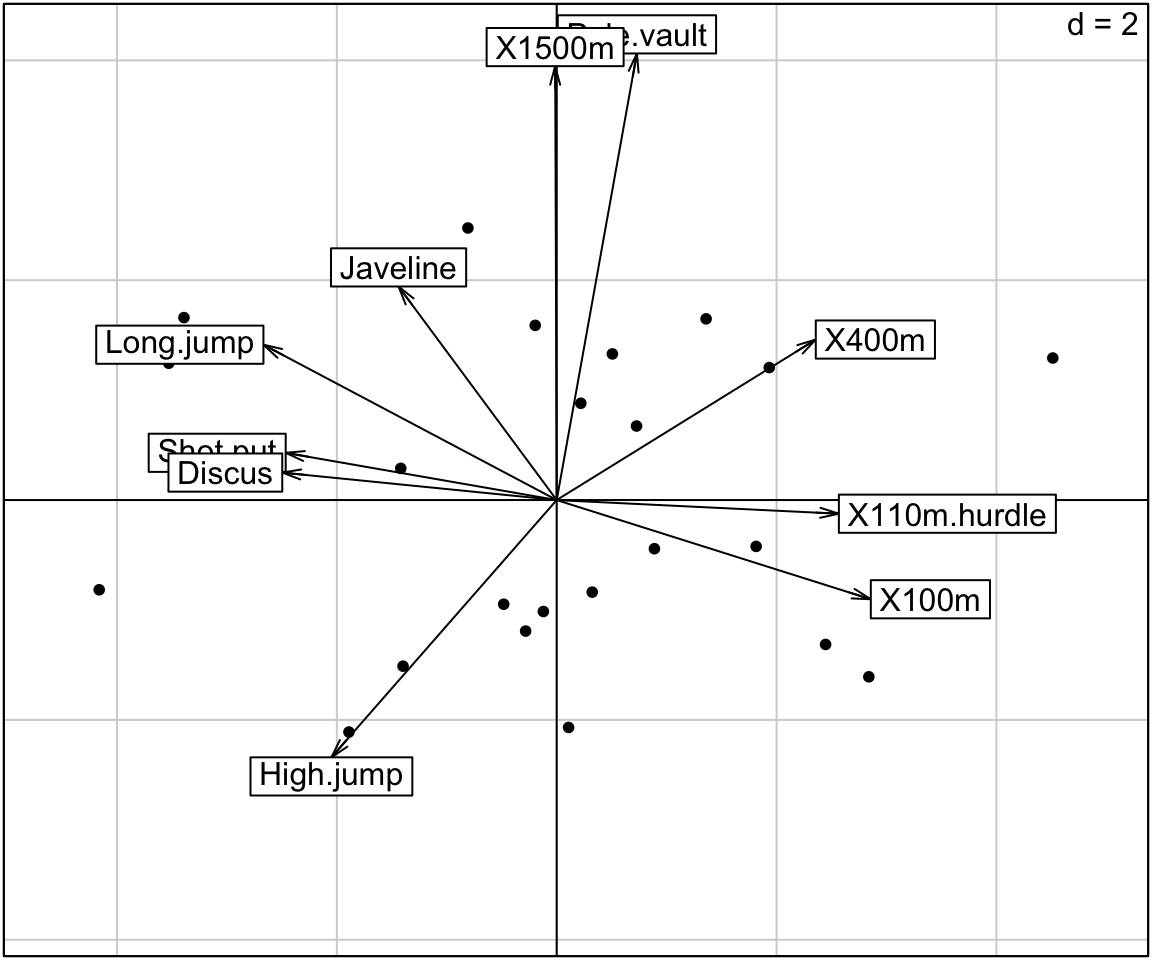
## NULLAccess to the PCA results
library(factoextra)
# Eigenvalues
eig.val <- get_eigenvalue(res.pca)
eig.val

# Results for Variables
res.var <- get_pca_var(res.pca)
res.var$coord          # Coordinates
res.var$contrib        # Contributions to the PCs
res.var$cos2           # Quality of representation
# Results for individuals
res.ind <- get_pca_ind(res.pca)
res.ind$coord          # Coordinates
res.ind$contrib        # Contributions to the PCs
res.ind$cos2           # Quality of representation
Predict using PCA
In this section, we’ll show how to predict the coordinates of supplementary individuals and variables using only the information provided by the previously performed PCA.
Supplementary individuals
- Data: rows 24 to 27 and columns 1 to to 10 [in decathlon2 data sets]. The new data must contain columns (variables) with the same names and in the same order as the active data used to compute PCA.
# Data for the supplementary individuals
ind.sup <- decathlon2[24:27, 1:10]
ind.sup[, 1:6]
## X100m Long.jump Shot.put High.jump X400m X110m.hurdle
## KARPOV 11.0 7.30 14.8 2.04 48.4 14.1
## WARNERS 11.1 7.60 14.3 1.98 48.7 14.2
## Nool 10.8 7.53 14.3 1.88 48.8 14.8
## Drews 10.9 7.38 13.1 1.88 48.5 14.0- Predict the coordinates of new individuals data.
ind.sup.coord <- suprow(res.pca, ind.sup) %>%
  .$lisup
ind.sup.coord[, 1:4]
## Axis1 Axis2 Axis3 Axis4
## KARPOV -0.795 0.7795 1.633 1.724
## WARNERS 0.386 -0.1216 1.739 -0.706
## Nool 0.559 1.9775 0.483 -2.278
## Drews 1.109 0.0174 3.049 -1.534- Graph of individuals including the supplementary individuals:
# Plot of active individuals
p <- fviz_pca_ind(res.pca, repel = TRUE)
# Add supplementary individuals
fviz_add(p, ind.sup.coord, color ="blue")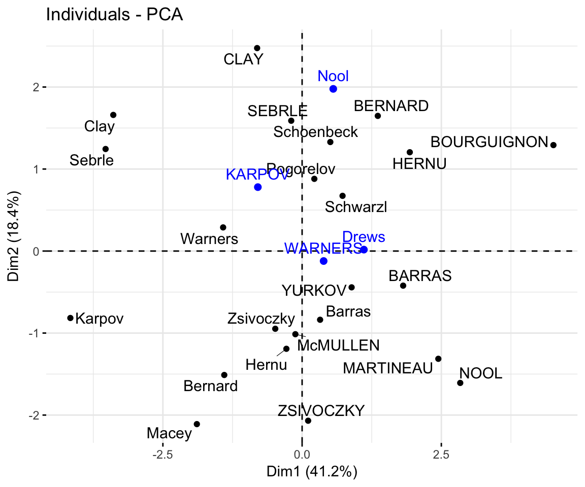
Supplementary variables
Qualitative / categorical variables
The data sets decathlon2 contain a supplementary qualitative variable at columns 13 corresponding to the type of competitions.
Qualitative / categorical variables can be used to color individuals by groups. The grouping variable should be of same length as the number of active individuals (here 23).
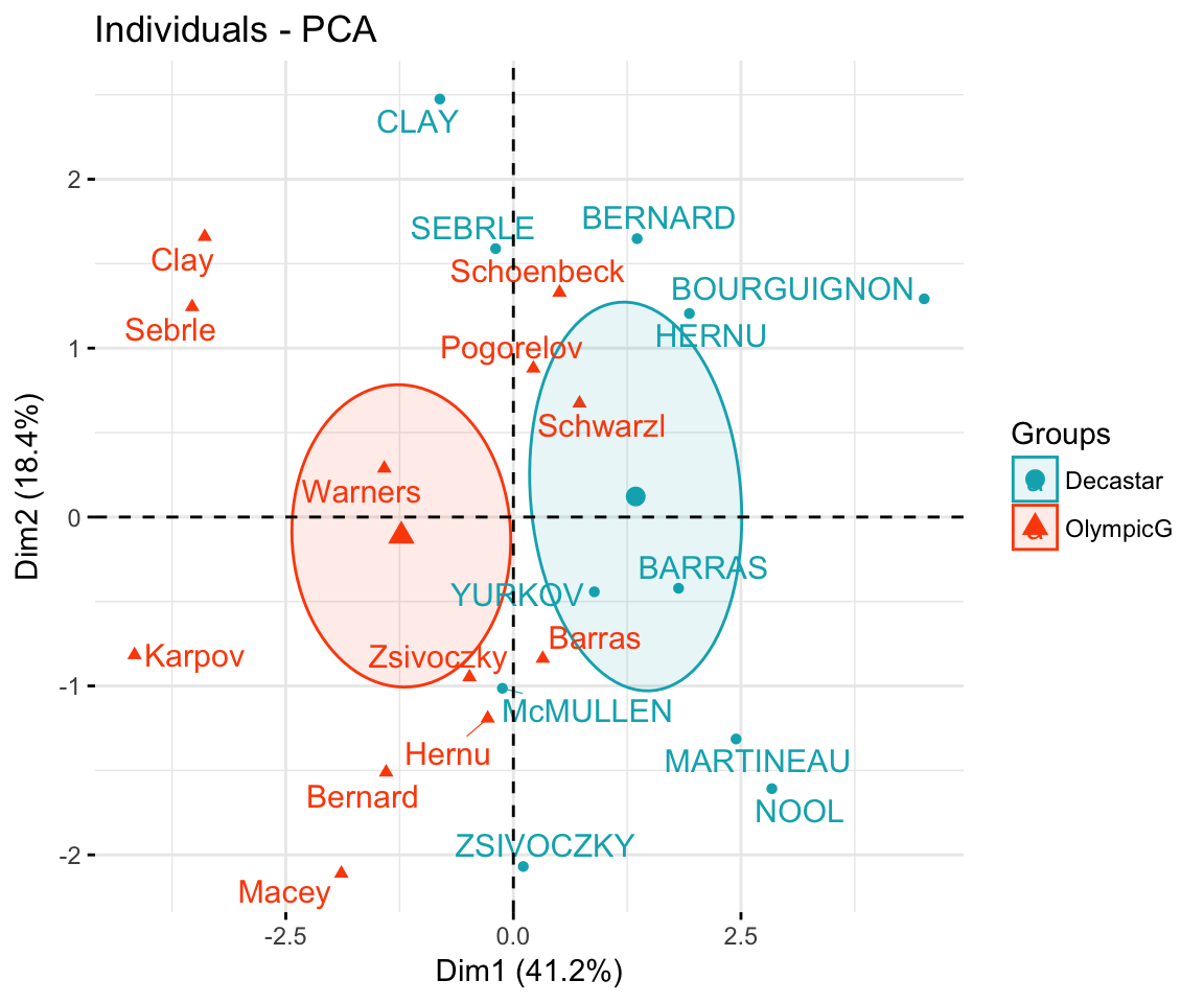
- factoextra-based plots
groups <- as.factor(decathlon2$Competition[1:23])
fviz_pca_ind(res.pca,
             col.ind = groups, # color by groups
             palette = c("#00AFBB",  "#FC4E07"),
             addEllipses = TRUE, # Concentration ellipses
             ellipse.type = "confidence",
             legend.title = "Groups",
             repel = TRUE
             )
- ade4-based plots:
groups <- as.factor(decathlon2$Competition[1:23])
s.class(res.pca$li,
        fac = groups,  # color by groups
        col = c("#00AFBB",  "#FC4E07")
        )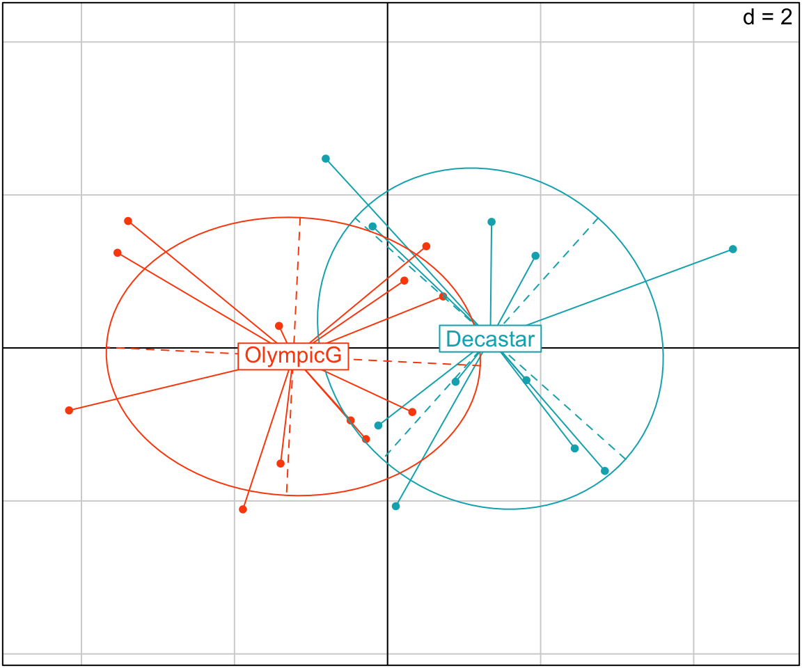
# Biplot
res <- scatter(res.pca, clab.row = 0, posieig = "none")
s.class(res.pca$li,
        fac = groups,
        col = c("#00AFBB",  "#FC4E07"),
        add.plot = TRUE,         # Add onto the scatter plot
        cstar = 0,               # Remove stars
        cellipse = 0             # Remove ellipses
        )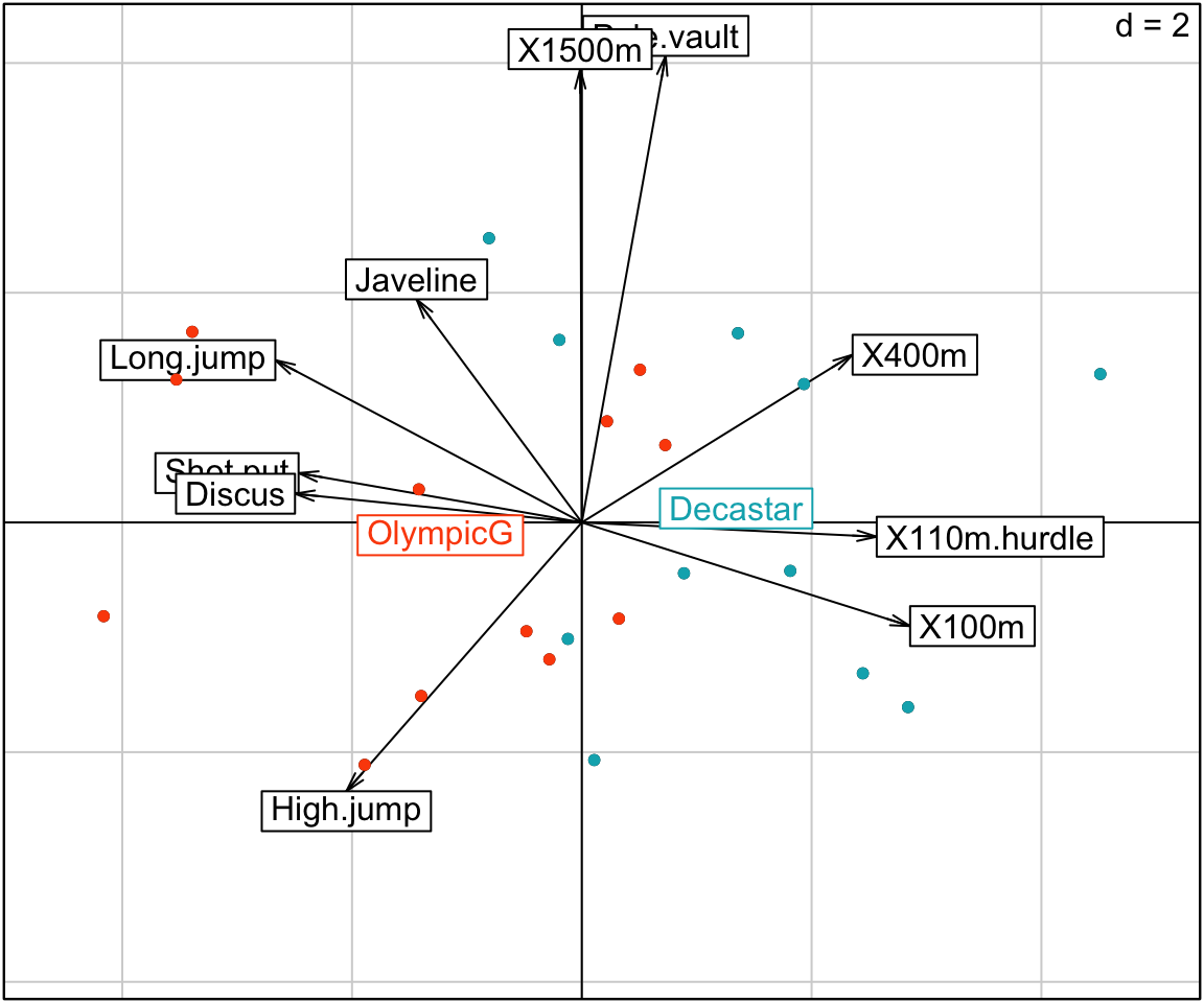
Quantitative variables
Data: columns 11:12. Should be of same length as the number of active individuals (here 23)
quanti.sup <- decathlon2[1:23, 11:12, drop = FALSE]
head(quanti.sup)
## Rank Points
## SEBRLE 1 8217
## CLAY 2 8122
## BERNARD 4 8067
## YURKOV 5 8036
## ZSIVOCZKY 7 8004
## McMULLEN 8 7995The coordinates of a given quantitative variable are calculated as the correlation between the quantitative variables and the principal components.
# Predict coordinates and compute cos2
quanti.coord <- supcol(res.pca, scale(quanti.sup)) %>%
  .$cosup
quanti.cos2 <- quanti.coord^2
# Graph of variables including supplementary variables
p <- fviz_pca_var(res.pca)
fviz_add(p, quanti.coord, color ="blue", geom="arrow")