Principal Component Analysis in R: prcomp vs princomp

kassambara | 08/10/2017 | 805974 | Comments (5) | Principal Component Methods in R: Practical Guide

This R tutorial describes how to perform a Principal Component Analysis (PCA) using the built-in R functions prcomp() and princomp(). You will learn how to predict new individuals and variables coordinates using PCA. We’ll also provide the theory behind PCA results.

Learn more about the basics and the interpretation of principal component analysis in our previous article: PCA - Principal Component Analysis Essentials.

PCA in R: prcomp vs princomp

Contents:

General methods for principal component analysis
prcomp() and princomp() functions
Package for PCA visualization
Demo data sets
Compute PCA in R using prcomp()
Access to the PCA results
Predict using PCA
- Supplementary individuals
- Supplementary variables
Theory behind PCA results
- PCA results for variables
- PCA results for individuals

Related Book:

Practical Guide to Principal Component Methods in R

General methods for principal component analysis

There are two general methods to perform PCA in R :

Spectral decomposition which examines the covariances / correlations between variables
Singular value decomposition which examines the covariances / correlations between individuals

The function princomp() uses the spectral decomposition approach. The functions prcomp() and PCA()[FactoMineR] use the singular value decomposition (SVD).

According to the R help, SVD has slightly better numerical accuracy. Therefore, the function prcomp() is preferred compared to princomp().

prcomp() and princomp() functions

The simplified format of these 2 functions are :

prcomp(x, scale = FALSE)
princomp(x, cor = FALSE, scores = TRUE)

Arguments for prcomp():

x: a numeric matrix or data frame
scale: a logical value indicating whether the variables should be scaled to have unit variance before the analysis takes place

Arguments for princomp():

x: a numeric matrix or data frame
cor: a logical value. If TRUE, the data will be centered and scaled before the analysis
scores: a logical value. If TRUE, the coordinates on each principal component are calculated

The elements of the outputs returned by the functions prcomp() and princomp() includes :

prcomp() name	princomp() name	Description
sdev	sdev	the standard deviations of the principal components
rotation	loadings	the matrix of variable loadings (columns are eigenvectors)
center	center	the variable means (means that were substracted)
scale	scale	the variable standard deviations (the scaling applied to each variable )
x	scores	The coordinates of the individuals (observations) on the principal components.

In the following sections, we’ll focus only on the function prcomp()

Package for PCA visualization

We’ll use the factoextra R package to create a ggplot2-based elegant visualization.

You can install it from CRAN:

install.packages("factoextra")

Or, install the latest developmental version from github:

if(!require(devtools)) install.packages("devtools")
devtools::install_github("kassambara/factoextra")

Load factoextra as follow:

library(factoextra)

Demo data sets

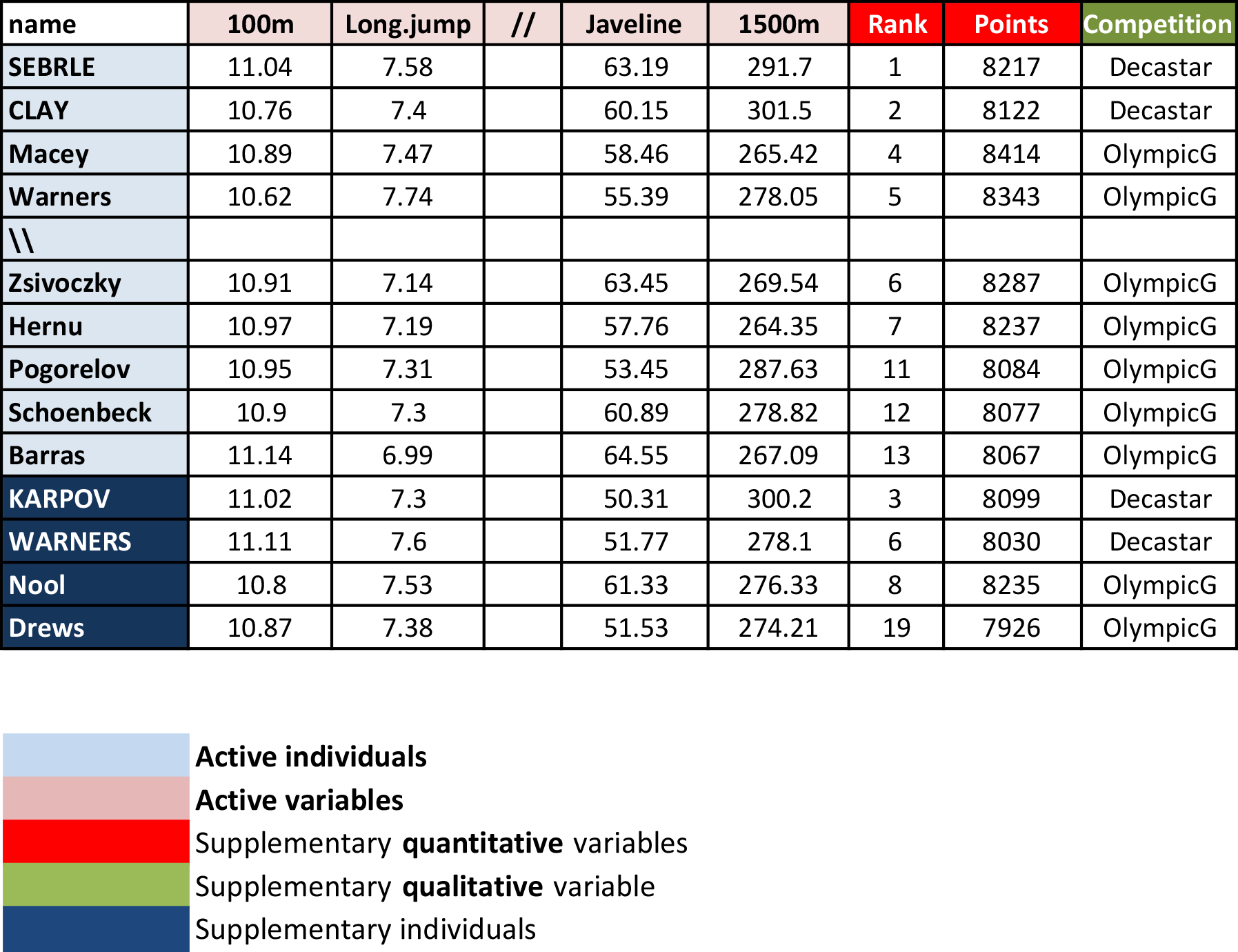
We’ll use the data sets decathlon2 [in factoextra], which has been already described at: PCA - Data format.

Briefly, it contains:

Active individuals (rows 1 to 23) and active variables (columns 1 to 10), which are used to perform the principal component analysis
Supplementary individuals (rows 24 to 27) and supplementary variables (columns 11 to 13), which coordinates will be predicted using the PCA information and parameters obtained with active individuals/variables.

Principal component analysis data format

Load the data and extract only active individuals and variables:

library("factoextra")
data(decathlon2)
decathlon2.active <- decathlon2[1:23, 1:10]
head(decathlon2.active[, 1:6])

##           X100m Long.jump Shot.put High.jump X400m X110m.hurdle
## SEBRLE     11.0      7.58     14.8      2.07  49.8         14.7
## CLAY       10.8      7.40     14.3      1.86  49.4         14.1
## BERNARD    11.0      7.23     14.2      1.92  48.9         15.0
## YURKOV     11.3      7.09     15.2      2.10  50.4         15.3
## ZSIVOCZKY  11.1      7.30     13.5      2.01  48.6         14.2
## McMULLEN   10.8      7.31     13.8      2.13  49.9         14.4

Compute PCA in R using prcomp()

In this section we’ll provide an easy-to-use R code to compute and visualize PCA in R using the prcomp() function and the factoextra package.

Load factoextra for visualization

library(factoextra)

Compute PCA

res.pca <- prcomp(decathlon2.active, scale = TRUE)

Visualize eigenvalues (scree plot). Show the percentage of variances explained by each principal component.

fviz_eig(res.pca)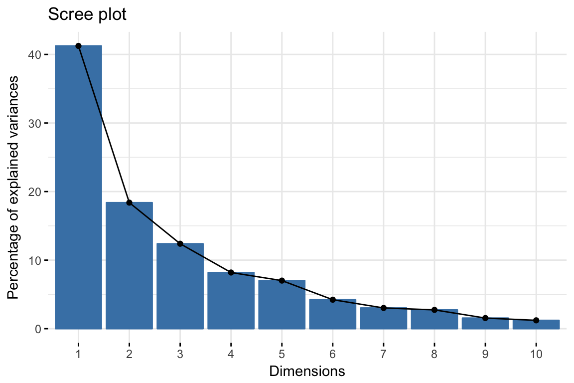

Graph of individuals. Individuals with a similar profile are grouped together.

fviz_pca_ind(res.pca,
             col.ind = "cos2", # Color by the quality of representation
             gradient.cols = c("#00AFBB", "#E7B800", "#FC4E07"),
             repel = TRUE     # Avoid text overlapping
             )

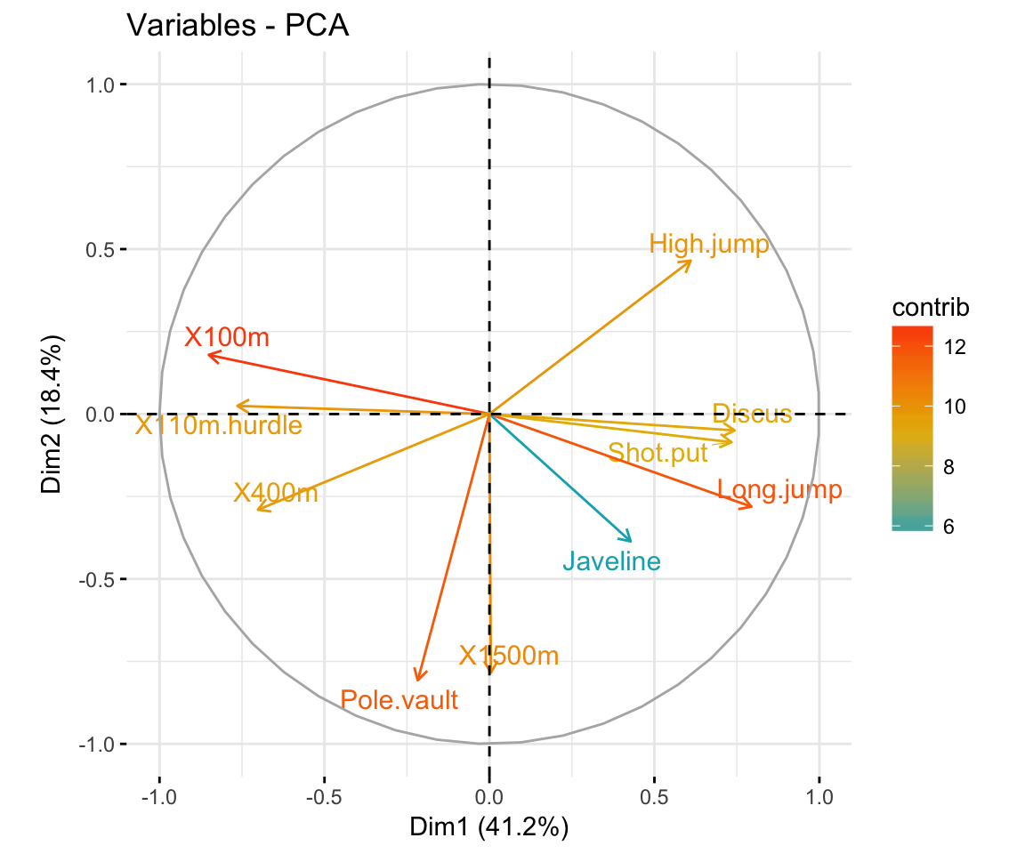
Graph of variables. Positive correlated variables point to the same side of the plot. Negative correlated variables point to opposite sides of the graph.

fviz_pca_var(res.pca,
             col.var = "contrib", # Color by contributions to the PC
             gradient.cols = c("#00AFBB", "#E7B800", "#FC4E07"),
             repel = TRUE     # Avoid text overlapping
             )

Biplot of individuals and variables

fviz_pca_biplot(res.pca, repel = TRUE,
                col.var = "#2E9FDF", # Variables color
                col.ind = "#696969"  # Individuals color
                )

Access to the PCA results

library(factoextra)
# Eigenvalues
eig.val <- get_eigenvalue(res.pca)
eig.val
  
# Results for Variables
res.var <- get_pca_var(res.pca)
res.var$coord          # Coordinates
res.var$contrib        # Contributions to the PCs
res.var$cos2           # Quality of representation 
# Results for individuals
res.ind <- get_pca_ind(res.pca)
res.ind$coord          # Coordinates
res.ind$contrib        # Contributions to the PCs
res.ind$cos2           # Quality of representation

Predict using PCA

In this section, we’ll show how to predict the coordinates of supplementary individuals and variables using only the information provided by the previously performed PCA.

Supplementary individuals

Data: rows 24 to 27 and columns 1 to to 10 [in decathlon2 data sets]. The new data must contain columns (variables) with the same names and in the same order as the active data used to compute PCA.

# Data for the supplementary individuals
ind.sup <- decathlon2[24:27, 1:10]
ind.sup[, 1:6]

##         X100m Long.jump Shot.put High.jump X400m X110m.hurdle
## KARPOV   11.0      7.30     14.8      2.04  48.4         14.1
## WARNERS  11.1      7.60     14.3      1.98  48.7         14.2
## Nool     10.8      7.53     14.3      1.88  48.8         14.8
## Drews    10.9      7.38     13.1      1.88  48.5         14.0

Predict the coordinates of new individuals data. Use the R base function predict():

ind.sup.coord <- predict(res.pca, newdata = ind.sup)
ind.sup.coord[, 1:4]

##            PC1    PC2   PC3    PC4
## KARPOV   0.777 -0.762 1.597  1.686
## WARNERS -0.378  0.119 1.701 -0.691
## Nool    -0.547 -1.934 0.472 -2.228
## Drews   -1.085 -0.017 2.982 -1.501

Graph of individuals including the supplementary individuals:

# Plot of active individuals
p <- fviz_pca_ind(res.pca, repel = TRUE)
# Add supplementary individuals
fviz_add(p, ind.sup.coord, color ="blue")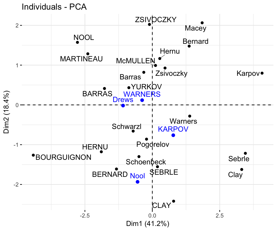

The predicted coordinates of individuals can be manually calculated as follow:

Center and scale the new individuals data using the center and the scale of the PCA
Calculate the predicted coordinates by multiplying the scaled values with the eigenvectors (loadings) of the principal components.

The R code below can be used :

# Centering and scaling the supplementary individuals
ind.scaled <- scale(ind.sup, 
                    center = res.pca$center,
                    scale = res.pca$scale)
# Coordinates of the individividuals
coord_func <- function(ind, loadings){
  r <- loadings*ind
  apply(r, 2, sum)
}
pca.loadings <- res.pca$rotation
ind.sup.coord <- t(apply(ind.scaled, 1, coord_func, pca.loadings ))
ind.sup.coord[, 1:4]

##            PC1    PC2   PC3    PC4
## KARPOV   0.777 -0.762 1.597  1.686
## WARNERS -0.378  0.119 1.701 -0.691
## Nool    -0.547 -1.934 0.472 -2.228
## Drews   -1.085 -0.017 2.982 -1.501

Supplementary variables

Qualitative / categorical variables

The data sets decathlon2 contain a supplementary qualitative variable at columns 13 corresponding to the type of competitions.

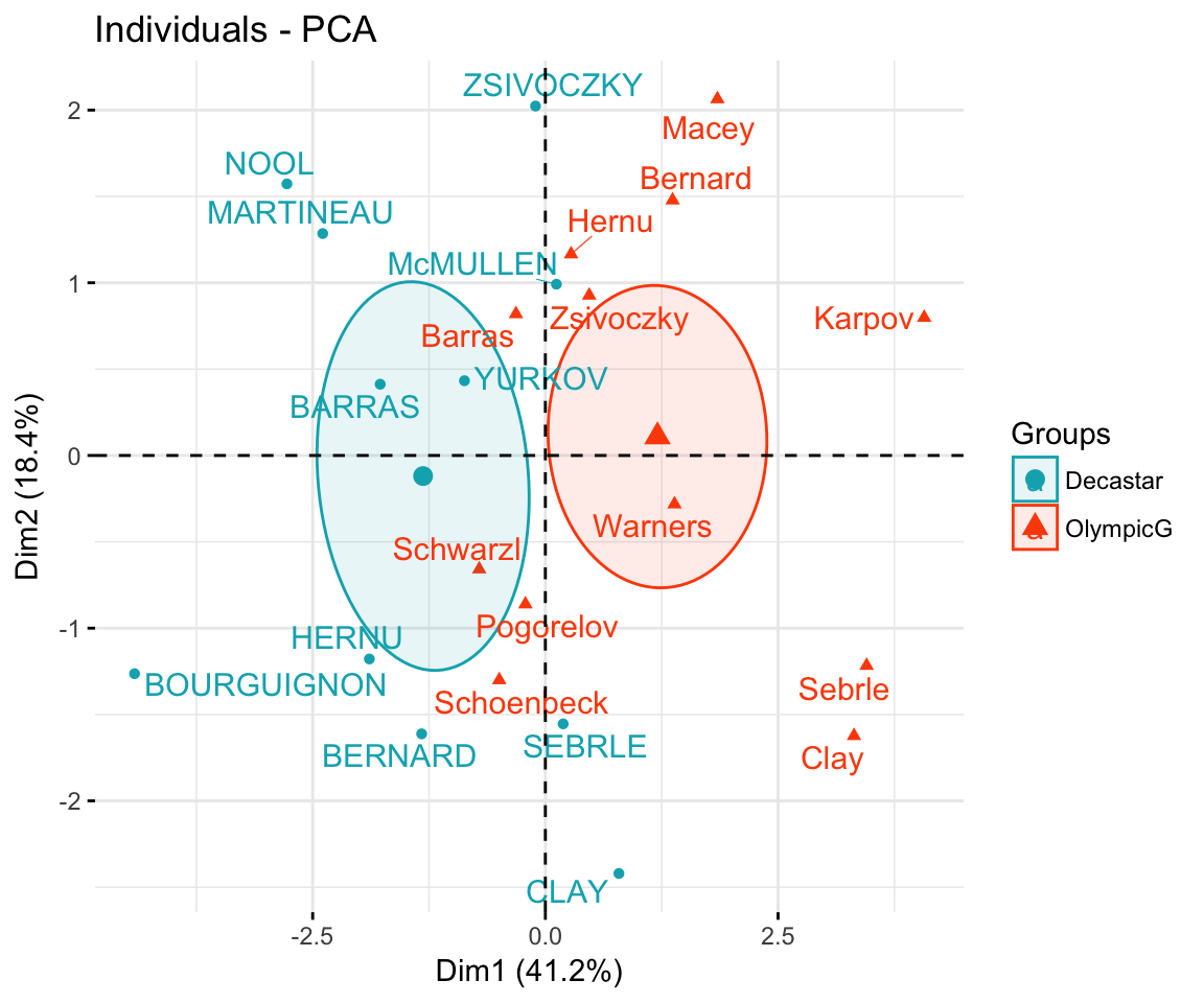
Qualitative / categorical variables can be used to color individuals by groups. The grouping variable should be of same length as the number of active individuals (here 23).

groups <- as.factor(decathlon2$Competition[1:23])
fviz_pca_ind(res.pca,
             col.ind = groups, # color by groups
             palette = c("#00AFBB",  "#FC4E07"),
             addEllipses = TRUE, # Concentration ellipses
             ellipse.type = "confidence",
             legend.title = "Groups",
             repel = TRUE
             )

Calculate the coordinates for the levels of grouping variables. The coordinates for a given group is calculated as the mean coordinates of the individuals in the group.

library(magrittr) # for pipe %>%
library(dplyr)   # everything else
# 1. Individual coordinates
res.ind <- get_pca_ind(res.pca)
# 2. Coordinate of groups
coord.groups <- res.ind$coord %>%
  as_data_frame() %>%
  select(Dim.1, Dim.2) %>%
  mutate(competition = groups) %>%
  group_by(competition) %>%
  summarise(
    Dim.1 = mean(Dim.1),
    Dim.2 = mean(Dim.2)
    )
coord.groups

## # A tibble: 2 x 3
##   competition Dim.1  Dim.2
##           
## 1    Decastar -1.31 -0.119
## 2    OlympicG  1.20  0.109

Quantitative variables

Data: columns 11:12. Should be of same length as the number of active individuals (here 23)

quanti.sup <- decathlon2[1:23, 11:12, drop = FALSE]
head(quanti.sup)

##           Rank Points
## SEBRLE       1   8217
## CLAY         2   8122
## BERNARD      4   8067
## YURKOV       5   8036
## ZSIVOCZKY    7   8004
## McMULLEN     8   7995

The coordinates of a given quantitative variable are calculated as the correlation between the quantitative variables and the principal components.

# Predict coordinates and compute cos2
quanti.coord <- cor(quanti.sup, res.pca$x)
quanti.cos2 <- quanti.coord^2
# Graph of variables including supplementary variables
p <- fviz_pca_var(res.pca)
fviz_add(p, quanti.coord, color ="blue", geom="arrow")

Theory behind PCA results

PCA results for variables

Here we’ll show how to calculate the PCA results for variables: coordinates, cos2 and contributions:

var.coord = loadings * the component standard deviations
var.cos2 = var.coord^2
var.contrib. The contribution of a variable to a given principal component is (in percentage) : (var.cos2 * 100) / (total cos2 of the component)

# Helper function 
#::::::::::::::::::::::::::::::::::::::::
var_coord_func <- function(loadings, comp.sdev){
  loadings*comp.sdev
}
# Compute Coordinates
#::::::::::::::::::::::::::::::::::::::::
loadings <- res.pca$rotation
sdev <- res.pca$sdev
var.coord <- t(apply(loadings, 1, var_coord_func, sdev)) 
head(var.coord[, 1:4])

##                 PC1     PC2    PC3     PC4
## X100m        -0.851  0.1794 -0.302  0.0336
## Long.jump     0.794 -0.2809  0.191 -0.1154
## Shot.put      0.734 -0.0854 -0.518  0.1285
## High.jump     0.610  0.4652 -0.330  0.1446
## X400m        -0.702 -0.2902 -0.284  0.4308
## X110m.hurdle -0.764  0.0247 -0.449 -0.0169

# Compute Cos2
#::::::::::::::::::::::::::::::::::::::::
var.cos2 <- var.coord^2
head(var.cos2[, 1:4])

##                PC1      PC2    PC3      PC4
## X100m        0.724 0.032184 0.0909 0.001127
## Long.jump    0.631 0.078881 0.0363 0.013315
## Shot.put     0.539 0.007294 0.2679 0.016504
## High.jump    0.372 0.216424 0.1090 0.020895
## X400m        0.492 0.084203 0.0804 0.185611
## X110m.hurdle 0.584 0.000612 0.2015 0.000285

# Compute contributions
#::::::::::::::::::::::::::::::::::::::::
comp.cos2 <- apply(var.cos2, 2, sum)
contrib <- function(var.cos2, comp.cos2){var.cos2*100/comp.cos2}
var.contrib <- t(apply(var.cos2,1, contrib, comp.cos2))
head(var.contrib[, 1:4])

##                PC1     PC2   PC3     PC4
## X100m        17.54  1.7505  7.34  0.1376
## Long.jump    15.29  4.2904  2.93  1.6249
## Shot.put     13.06  0.3967 21.62  2.0141
## High.jump     9.02 11.7716  8.79  2.5499
## X400m        11.94  4.5799  6.49 22.6509
## X110m.hurdle 14.16  0.0333 16.26  0.0348

PCA results for individuals

ind.coord = res.pca$x
Cos2 of individuals. Two steps:
- Calculate the square distance between each individual and the PCA center of gravity: d2 = [(var1_ind_i - mean_var1)/sd_var1]^2 + …+ [(var10_ind_i - mean_var10)/sd_var10]^2 + …+..
- Calculate the cos2 as ind.coord^2/d2
Contributions of individuals to the principal components: 100 * (1 / number_of_individuals)*(ind.coord^2 / comp_sdev^2). Note that the sum of all the contributions per column is 100

# Coordinates of individuals
#::::::::::::::::::::::::::::::::::
ind.coord <- res.pca$x
head(ind.coord[, 1:4])

##              PC1    PC2    PC3     PC4
## SEBRLE     0.191 -1.554 -0.628  0.0821
## CLAY       0.790 -2.420  1.357  1.2698
## BERNARD   -1.329 -1.612 -0.196 -1.9209
## YURKOV    -0.869  0.433 -2.474  0.6972
## ZSIVOCZKY -0.106  2.023  1.305 -0.0993
## McMULLEN   0.119  0.992  0.844  1.3122

# Cos2 of individuals
#:::::::::::::::::::::::::::::::::
# 1. square of the distance between an individual and the
# PCA center of gravity
center <- res.pca$center
scale<- res.pca$scale
getdistance <- function(ind_row, center, scale){
  return(sum(((ind_row-center)/scale)^2))
  }
d2 <- apply(decathlon2.active,1,getdistance, center, scale)
# 2. Compute the cos2. The sum of each row is 1
cos2 <- function(ind.coord, d2){return(ind.coord^2/d2)}
ind.cos2 <- apply(ind.coord, 2, cos2, d2)
head(ind.cos2[, 1:4])

##               PC1    PC2     PC3     PC4
## SEBRLE    0.00753 0.4975 0.08133 0.00139
## CLAY      0.04870 0.4570 0.14363 0.12579
## BERNARD   0.19720 0.2900 0.00429 0.41182
## YURKOV    0.09611 0.0238 0.77823 0.06181
## ZSIVOCZKY 0.00157 0.5764 0.23975 0.00139
## McMULLEN  0.00218 0.1522 0.11014 0.26649

# Contributions of individuals
#:::::::::::::::::::::::::::::::
contrib <- function(ind.coord, comp.sdev, n.ind){
  100*(1/n.ind)*ind.coord^2/comp.sdev^2
}
ind.contrib <- t(apply(ind.coord, 1, contrib, 
                       res.pca$sdev, nrow(ind.coord)))
head(ind.contrib[, 1:4])

##              PC1    PC2    PC3     PC4
## SEBRLE    0.0385  5.712  1.385  0.0357
## CLAY      0.6581 13.854  6.460  8.5557
## BERNARD   1.8627  6.144  0.135 19.5783
## YURKOV    0.7969  0.443 21.476  2.5794
## ZSIVOCZKY 0.0118  9.682  5.975  0.0523
## McMULLEN  0.0148  2.325  2.497  9.1353

Last update : 08/10/2017

0 Note

Enjoyed this article? Give us 5 stars (just above this text block)! Reader needs to be STHDA member for voting. I’d be very grateful if you’d help it spread by emailing it to a friend, or sharing it on Twitter, Facebook or Linked In.

Show me some love with the like buttons below... Thank you and please don't forget to share and comment below!!

Avez vous aimé cet article? Donnez nous 5 étoiles (juste au dessus de ce block)! Vous devez être membre pour voter. Je vous serais très reconnaissant si vous aidiez à sa diffusion en l'envoyant par courriel à un ami ou en le partageant sur Twitter, Facebook ou Linked In.

Montrez-moi un peu d'amour avec les like ci-dessous ... Merci et n'oubliez pas, s'il vous plaît, de partager et de commenter ci-dessous!

Recommended for You!

Machine Learning Essentials: Practical Guide in R

Practical Guide to Cluster Analysis in R

Practical Guide to Principal Component Methods in R

R Graphics Essentials for Great Data Visualization

Network Analysis and Visualization in R

More books on R and data science

Recommended for you

This section contains the best data science and self-development resources to help you on your path.

Books - Data Science

Our Books

Practical Guide to Cluster Analysis in R by A. Kassambara (Datanovia)
Practical Guide To Principal Component Methods in R by A. Kassambara (Datanovia)
Machine Learning Essentials: Practical Guide in R by A. Kassambara (Datanovia)
R Graphics Essentials for Great Data Visualization by A. Kassambara (Datanovia)
GGPlot2 Essentials for Great Data Visualization in R by A. Kassambara (Datanovia)
Network Analysis and Visualization in R by A. Kassambara (Datanovia)
Practical Statistics in R for Comparing Groups: Numerical Variables by A. Kassambara (Datanovia)
Inter-Rater Reliability Essentials: Practical Guide in R by A. Kassambara (Datanovia)

Others

R for Data Science: Import, Tidy, Transform, Visualize, and Model Data by Hadley Wickham & Garrett Grolemund
Hands-On Machine Learning with Scikit-Learn, Keras, and TensorFlow: Concepts, Tools, and Techniques to Build Intelligent Systems by Aurelien Géron
Practical Statistics for Data Scientists: 50 Essential Concepts by Peter Bruce & Andrew Bruce
Hands-On Programming with R: Write Your Own Functions And Simulations by Garrett Grolemund & Hadley Wickham
An Introduction to Statistical Learning: with Applications in R by Gareth James et al.
Deep Learning with R by François Chollet & J.J. Allaire
Deep Learning with Python by François Chollet

Comments

You are not authorized to post a comment

Comment

Melisa

Member

#911 04/01/2021 at 04h32

Hi! thank you very much for this guide is amazing.. I would like to ask you how you choose the outliers from this data?

Comment

Alam

Visitor

#642 11/11/2018 at 12h13

Thank you very much for this nice tutorial.

I have one problem. How to italize the variable name in PCA correlation circle plot.

I am looking forward to hearing.

Comment

Mike

Visitor

#633 10/18/2018 at 09h57

Sorry to Necro this thread, but I have to say, what a fantastic guide! It has come in very helpful. Thank you so much for putting this together. I'm curious if anyone else has had trouble plotting the ellipses?

When I try to run the code under the "Qualitative / categorical variables" section I am returned with this error:
<Computation failed in `stat_conf_ellipse()`: missing value where TRUE/FALSE needed>

I looked up Stat_conf_ellipse to learn more about it, loaded ggpubr, and added it to my command. After running it, the plot appears with the correct groupings but no ellipses, along with the following error:
<Error in .check_axes(axes, .length = 2) : axes should be of length 2>

My plot scale is 2 so this makes sense, the length of the axes needs to fit in the plot, so less than 2. I change this and retry, and then I get <Error in check_axes(axes, .length = 0.5) : could not find function "check_axes",>.

I have tried numerous combinations using "stat_conf_ellipse" and none of them have worked. I nested it in the fviz_pca_ind command, added it on the end with a +, add and remove functions from the stat_conf_ellipse help page.....nothing I try is working.

Does anyone have experience with this and thoughts on why it might be failing? Again, it plots fine with proper groups and colors, but no ellipses. Here was the last iteration of code I had:

fviz_pca_ind(mydata.pca, col.ind = groups, palette = c("#00AFBB", "#FC4E07", "#bb00a8"),addEllipses = TRUE, ellipse.type = "confidence",legend.title = "Groups",repel = TRUE, stat_conf_ellipse(position = "identity", na.rm = FALSE, show.legend = NA, inherit.aes = true, level = 0.95, npoint = 100, bary = true))

The error on the above code: Error in .check_axes(axes, .length = 2) : axes should be of length 2

Thanks for any help!

Comment

Konig

Visitor

#303 11/19/2017 at 17h46

Hi there,

Could you help me out interpreting the correlation of Rank and Points against the PCs? Is there a way to determine whether these are statistically significant to the PCA results? Thanks!

Comment

Visitor

#289 11/07/2017 at 19h13

Want to learn about PCA

STAY UPDATED

Articles - Principal Component Methods in R: Practical Guide