


MCA in R Using FactoMineR: Quick Scripts and Videos
This article presents quick start R code and video series for computing MCA (Multiple Correspondence Analysis) in R, using the FactoMineR package. Recall that MCA is used for analyzing multivarariate data sets containing categorical variables, such as survey data.
Contents:
Quick start R code
- Install FactoMineR package:
install.packages("FactoMineR")- Compute MCA using the demo data set
poison[in FactoMineR]. This data set refers to a survey carried out on a sample of children of primary school who suffered from food poisoning. They were asked about their symptoms and about what they ate.
library(FactoMineR)
data("poison")
res.mca <- MCA(poison,
              quanti.sup = 1:2, # Supplementary quantitative variable
              quali.sup = 3:4,  # Supplementary qualitative variable
              graph=FALSE)
Key terms:
- Active individuals and variables are used during the MCA.
- Supplementary individuals and variables: their coordinates will be predicted after the MCA.
- Visualize eigenvalues (scree plot). Show the percentage of variances explained by each principal component.
eig.val <- res.mca$eig
barplot(eig.val[, 2],
        names.arg = 1:nrow(eig.val),
        main = "Variances Explained by Dimensions (%)",
        xlab = "Principal Dimensions",
        ylab = "Percentage of variances",
        col ="steelblue")
# Add connected line segments to the plot
lines(x = 1:nrow(eig.val), eig.val[, 2],
      type = "b", pch = 19, col = "red")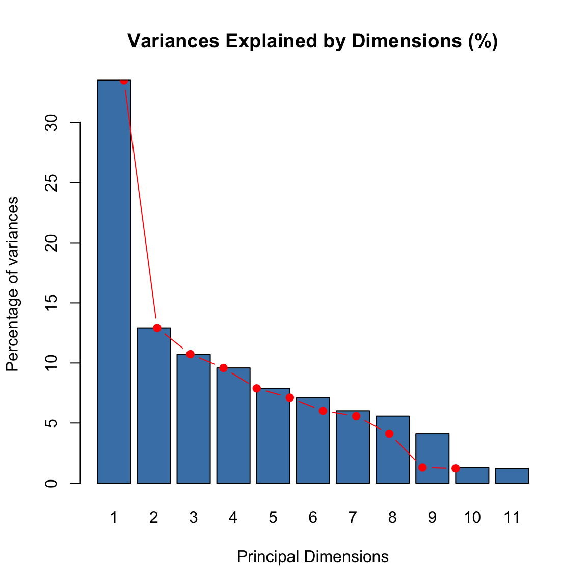
- Biplot of individuals and variables showing the link between them.
plot(res.mca, autoLab = "yes")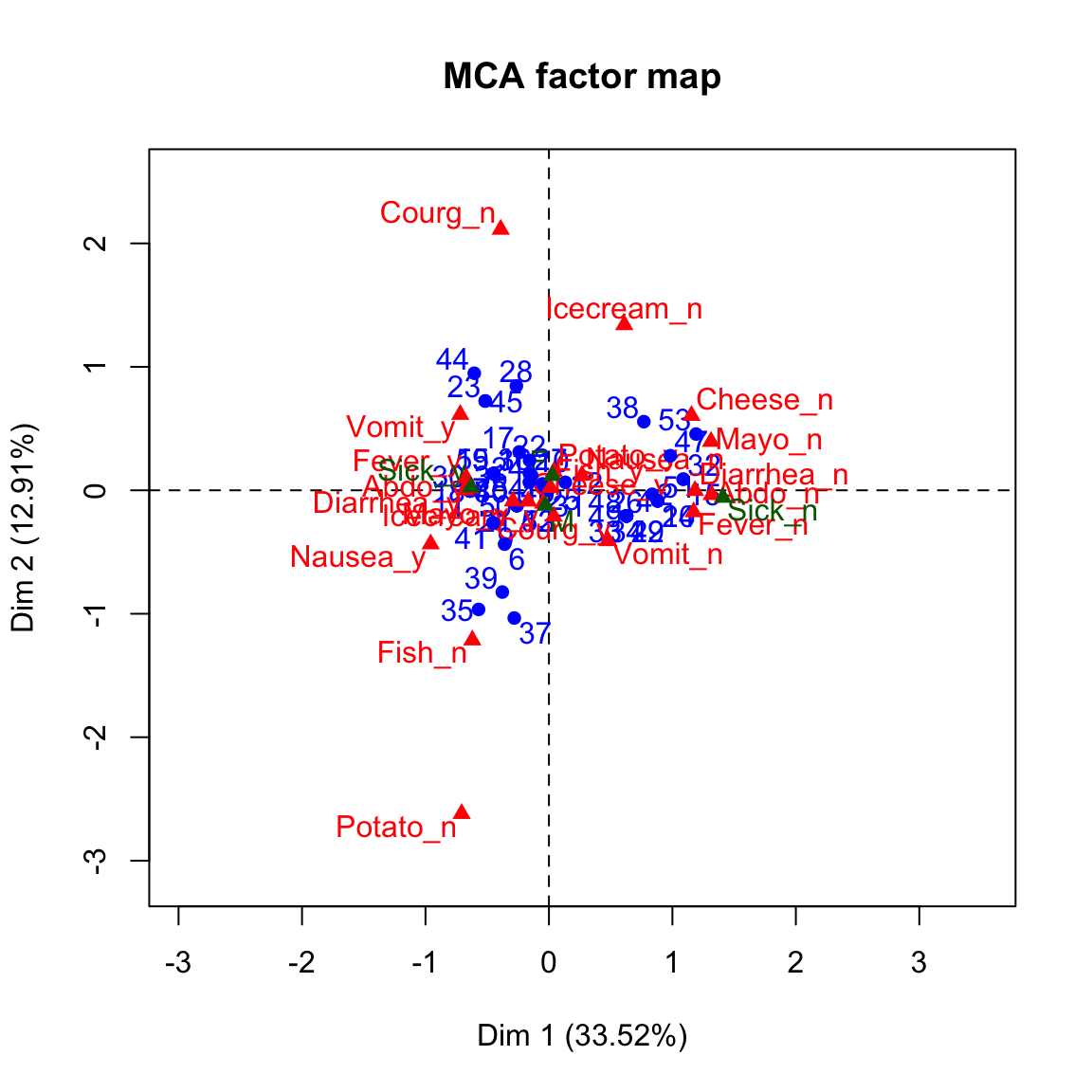
Blue: Individualsred: Variablesdark.green: Qualitative supplementary variable color
- Graph of individuals. Individuals with a similar profile are grouped together. Use the argument
invisibleto hide active and supplementary variables on the plot.
plot(res.mca,
     invisible = c("var", "quali.sup", "quanti.sup"),
     cex = 0.8,
     autoLab = "yes")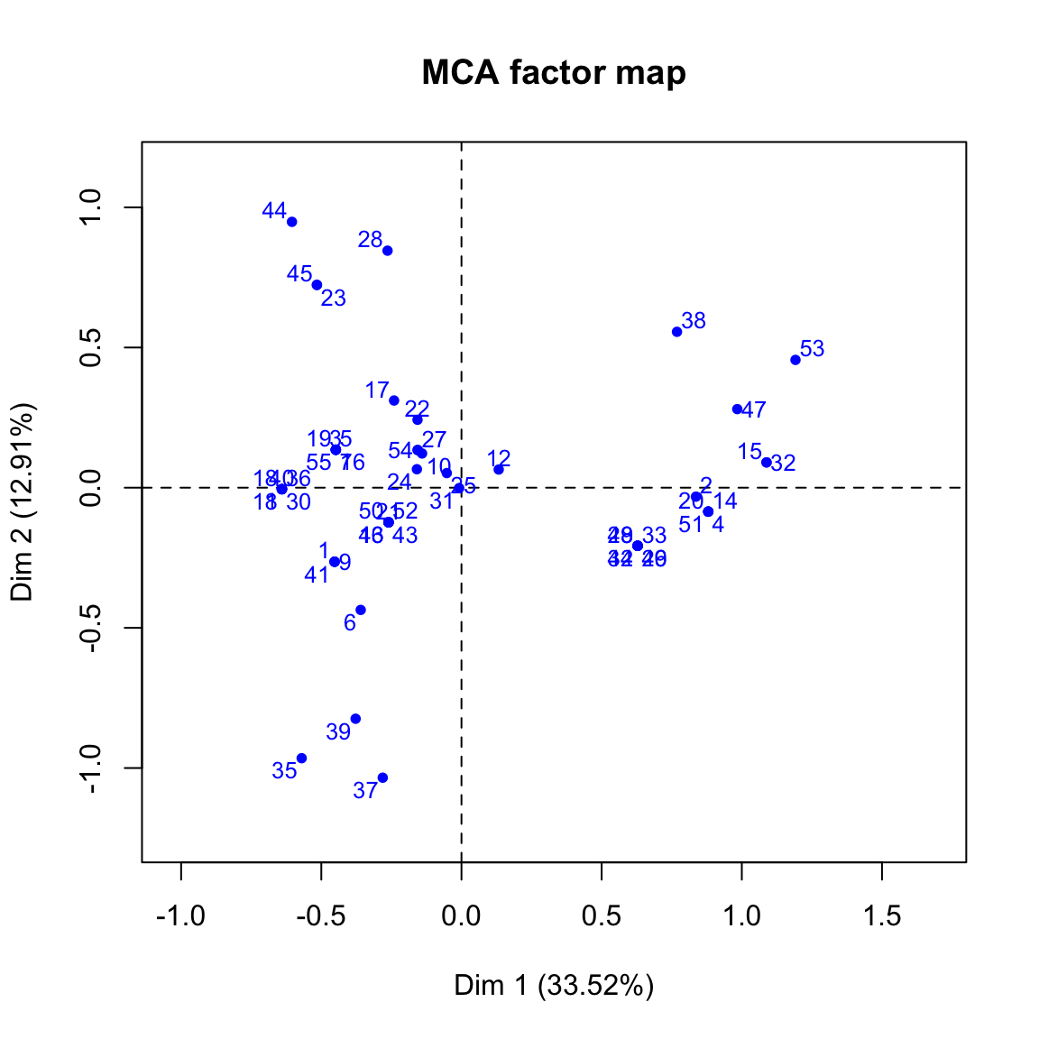
- Graph of active variables. Use the argument
invisibleto hide individuals and supplementary variables on the plot
plot(res.mca,
     invisible = c("ind", "quali.sup", "quanti.sup"),
     cex = 0.8,
     autoLab = "yes")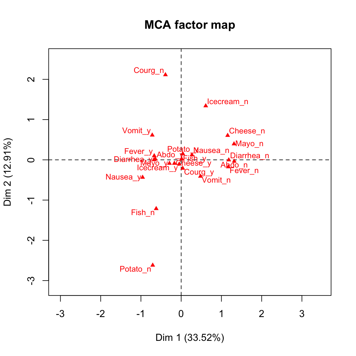
- Color individuals by groups and add confidence ellipses around the mean of groups.
plotellipses(res.mca, keepvar = c("Vomiting", "Fish"))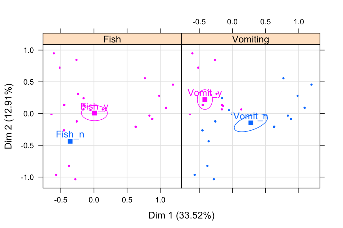
For ggplot2-based visualization, read this: MCA - Multiple Correspondence Analysis in R: Essentials
- Access to the results:
# Eigenvalues
res.mca$eig

# Results for active Variables
res.var <- res.mca$var
res.var$coord          # Coordinates
res.var$contrib        # Contributions to the PCs
res.var$cos2           # Quality of representation
# Results for qualitative supp. variables
res.mca$quali.sup
# Results for active individuals
res.ind <- res.mca$var
res.ind$coord          # Coordinates
res.ind$contrib        # Contributions to the PCs
res.ind$cos2           # Quality of representation
The following series of video explains the basics of MCA and show practical examples and interpretation in R.
Theory and key concepts
Data types
This video describes the data format and the goals of MCA.
Visualizing the point cloud of individuals
This video shows how to build the point cloud of rows/individuals and, how to interpret it using the variable’s categories.
Visualizing the cloud of categories
In this video, you’ll learn how to build point clouds of categories, as well as, how to get an optimal representation of them. You will discover the link between the optimal representation of individuals and the optimal representation of categories.
Interpretation
This video describes some interpretation aids, shared by all principal component methods. Additionally, it shows how to use supplementary information, including supplementary variables, in MCA.
Course video materials
MCA examples in R
MCA in practice with FactoMineR
Handling missing values
This video show how to handle missing values in MCA using missMDA and FactoMineR packages
MCA Graphical user interface: Factoshiny
Automatic interpretation: FactoInvestigate
The FactoInvestigate R package makes it possible to generate automatically a report for principal component analysis. Learn more in our previous article: FactoInvestigate R Package: Automatic Reports and Interpretation of Principal Component Analyses


