


PCA in R Using FactoMineR: Quick Scripts and Videos
This article starts by providing a quick start R code for computing PCA in R, using the FactoMineR, and continues by presenting series of PCA video courses (by François Husson).
Recall that PCA (Principal Component Analysis) is a multivariate data analysis method that allows us to summarize and visualize the information contained in a large data sets of quantitative variables.
In these video courses, the instructor François Husson, walks through the theory behind PCA (first 3 videos), to practical PCA examples in R programming language using the FactoMineR package. He also presents how to interpret the results.
François Husson, continues the course by presenting convenient solution to handle situations where the data contain missing values. This is made possible thanks to the missMDA R package.
Additionally, he presents the Factoshiny package, which provide an easy to use graphical interface to perform PCA. This is very useful for users with non advanced programming background.
He finishes by presenting the FactoInvestigate R package, which makes it easy to generate automatically a report - in HTML, PDF or Word formats - containing the PCA outputs and interpretation.
Contents:
Quick start R code
- Install FactoMineR package:
install.packages("FactoMineR")- Compute PCA using the demo data set USArrests. The data set contains statistics, in arrests per 100,000 residents for assault, murder, and rape in each of the 50 US states in 1973.
library(FactoMineR)
data("USArrests")
res.pca <- PCA(USArrests, graph = FALSE)- Visualize eigenvalues (scree plot). Show the percentage of variances explained by each principal component.
eig.val <- res.pca$eig
barplot(eig.val[, 2],
        names.arg = 1:nrow(eig.val),
        main = "Variances Explained by PCs (%)",
        xlab = "Principal Components",
        ylab = "Percentage of variances",
        col ="steelblue")
# Add connected line segments to the plot
lines(x = 1:nrow(eig.val), eig.val[, 2],
      type = "b", pch = 19, col = "red")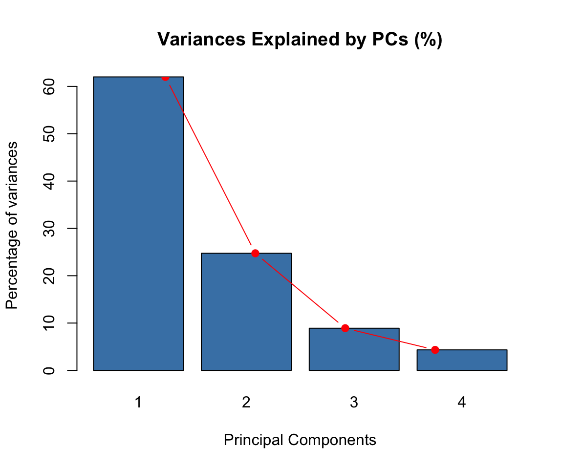
- Visualize the graph of individuals. Individuals with a similar profile are grouped together.
plot(res.pca, choix = "ind", autoLab = "yes")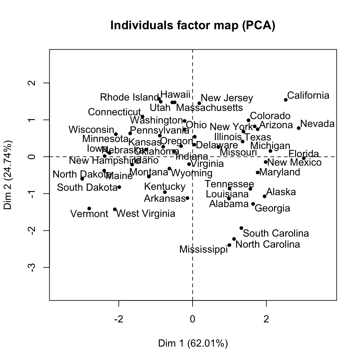
- Visualize the graph of variables. Positive correlated variables point to the same side of the plot. Negative correlated variables point to opposite sides of the graph.
plot(res.pca, choix = "var", autoLab = "yes")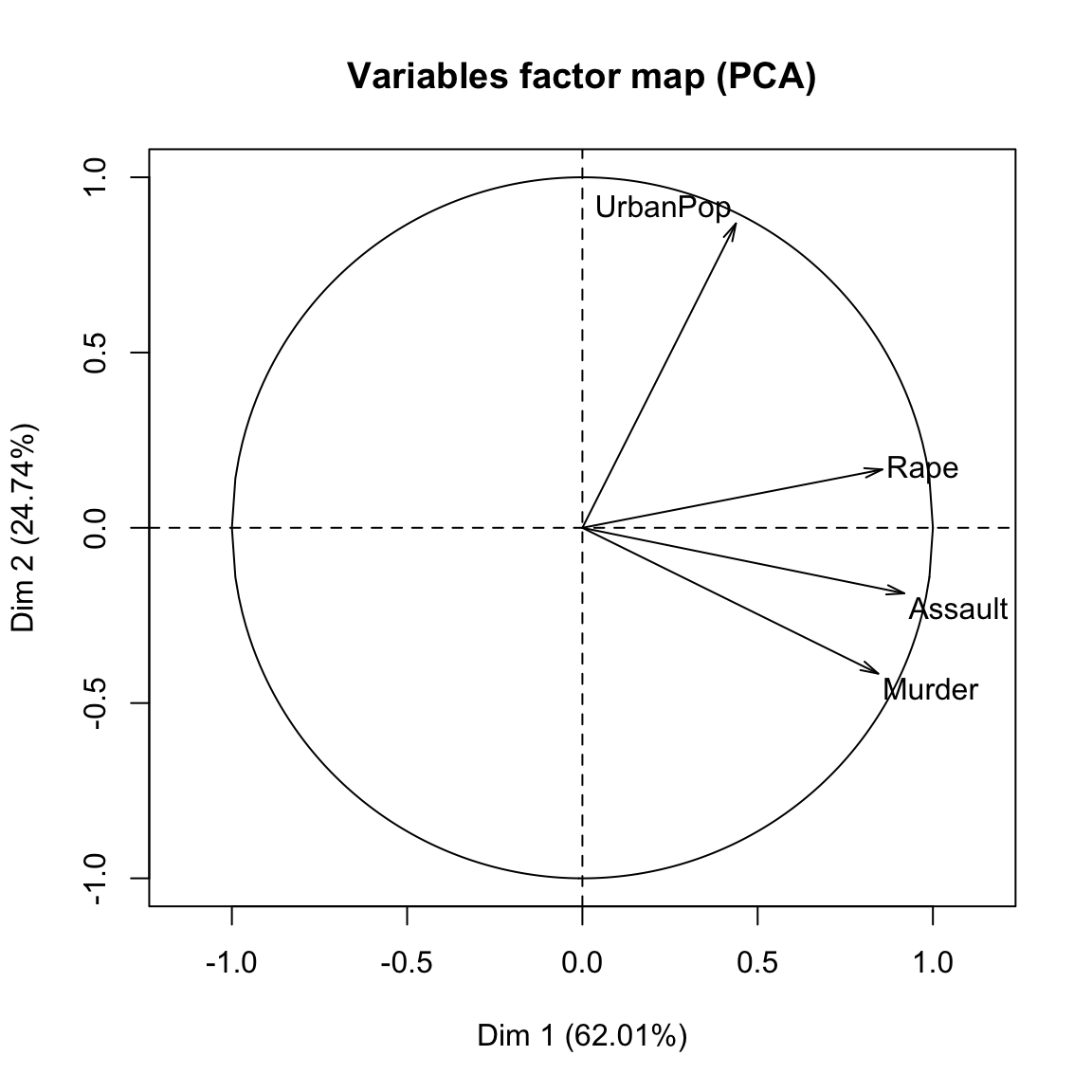
For ggplot2-based visualization, read this: PCA - Principal Component Analysis Essentials
- Access to the results:
# Eigenvalues
res.pca$eig

# Results for Variables
res.var <- res.pca$var
res.var$coord          # Coordinates
res.var$contrib        # Contributions to the PCs
res.var$cos2           # Quality of representation
# Results for individuals
res.ind <- res.pca$var
res.ind$coord          # Coordinates
res.ind$contrib        # Contributions to the PCs
res.ind$cos2           # Quality of representation
Theory and key concepts
Data types
This video presents the type of data to be used for principal component analysis and defines some useful notations. It introduces also the type of questions one can investigate with PCA.
Studying individuals and variables
This video presents how individuals and variables coordinates are calculated and visualized.
PCA interpretation
This video presents tips and tricks that help to interpret the output of PCA.
Course video materials
PCA examples in R
PCA in practice with FactoMineR
Handling missing values
This video show how to handle missing values in PCA using missMDA and FactoMineR packages
PCA Graphical user interface: Factoshiny
Automatic interpretation: FactoInvestigate
The FactoInvestigate R package makes it possible to generate automatically a report for principal component analysis. Learn more in our previous article: FactoInvestigate R Package: Automatic Reports and Interpretation of Principal Component Analyses


