Visualize NGS data with R and Bioconductor

Load packages and data

We’re going to use the RNA sequencing experiment in the passilaBamSubset package.

#biocLite("pasillaBamSubset")
#biocLite("TxDb.Dmelanogaster.UCSC.dm3.ensGene")
library(pasillaBamSubset)
#Genes annotated in transcript database
library(TxDb.Dmelanogaster.UCSC.dm3.ensGene)
#The 2 files of interest
fl1 <- untreated1_chr4()
fl2 <- untreated3_chr4()

fl1 and fl2 are bam file from RNA sequencing data of Drosophila.

Simple plot

library(GenomicRanges)

Note: if you are using Bioconductor version 14, paired with R 3.1, you should also load the following library. You do not need to load this library, and it will not be available to you, if you are using Bioconductor version 13, paired with R 3.0.x.

library(GenomicAlignments)

We read in the alignments from the file fl1. Then we use the coverage function to tally up the base pair coverage. We then extract the subset of coverage which overlaps our gene of interest (lgs gene), and convert this coverage from an RleList into a numeric vector. Rle objects are compressed, such that repeating numbers are stored as a number and a length.

# x is a class of GAlignments, Each row is a read
x <- readGAlignments(fl1)
#Coverage of the reads : this will generate a RleList
#Rle is a run-length encoding (week2)
xcov <- coverage(x)
xcov

## RleList of length 8
## $chr2L
## integer-Rle of length 23011544 with 1 run
##   Lengths: 23011544
##   Values :        0
## 
## $chr2R
## integer-Rle of length 21146708 with 1 run
##   Lengths: 21146708
##   Values :        0
## 
## $chr3L
## integer-Rle of length 24543557 with 1 run
##   Lengths: 24543557
##   Values :        0
## 
## $chr3R
## integer-Rle of length 27905053 with 1 run
##   Lengths: 27905053
##   Values :        0
## 
## $chr4
## integer-Rle of length 1351857 with 122061 runs
##   Lengths:  891   27    5   12   13   45 ...    3  106   75 1600   75 1659
##   Values :    0    1    2    3    4    5 ...    6    0    1    0    1    0
## 
## ...
## <3 more elements>

#Extract one element of the list
#we have zero coverage for the first 891 base pairs,
#and then we have coverage of one for 27 base pairs, etc.
xcov$chr4

## integer-Rle of length 1351857 with 122061 runs
##   Lengths:  891   27    5   12   13   45 ...    3  106   75 1600   75 1659
##   Values :    0    1    2    3    4    5 ...    6    0    1    0    1    0

#Let's zoom in now to range which is near this gene of interest, LGS.
z <- GRanges("chr4",IRanges(456500,466000))
# only available for Bioconductor 2.14
xcov[z]#subset the coverage of the region of interest

## RleList of length 1
## $chr4
## integer-Rle of length 9501 with 1775 runs
##   Lengths: 1252   10   52    4    7    2 ...   10    7   12  392   75 1041
##   Values :    0    2    3    4    5    6 ...    3    2    1    0    1    0

# Equivalent in Bioconductor 2.13
#xcov$chr4[ranges(z)]# Works for all version of Bioconductor
#Plot of the coverage arround the region of interest
xnum <- as.numeric(xcov$chr4[ranges(z)])#Uncompress the coverage
plot(xnum)

We can do the same for another file: So because fl2 is a paired in sequencing experiment, we now have pairs of reads which corresponds to one fragment.

y <- readGAlignmentPairs(fl2)
ycov <- coverage(y)
ynum <- as.numeric(ycov$chr4[ranges(z)])
plot(xnum, type="l", col="blue", lwd=2)
lines(ynum, col="red", lwd=2)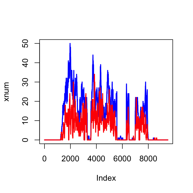

We can zoom in on a single exon, between the area of 6 000 base pairs:

plot(xnum, type="l", col="blue", lwd=2, xlim=c(6200,6600))
lines(ynum, col="red", lwd=2)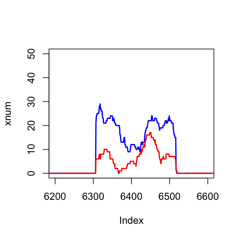

Extracting the gene of interest using the transcript database

Extract information about gene of interest.

Suppose we are interested in visualizing the gene lgs. We can extract it from the transcript database TxDb.Dmelanogaster.UCSC.dm3.ensGene on Bioconductor, but first we need to look up the Ensembl gene name. We will use the functions that we learned in the previous chapter.

# biocLite("biomaRt")
library(biomaRt)
#load the drosophila ensemble gene BioMart.
m <- useMart("ensembl", dataset = "dmelanogaster_gene_ensembl")
lf <- listFilters(m)
lf[grep("name", lf$description, ignore.case=TRUE),]

##                             name
## 1                chromosome_name
## 12  with_flybasename_translation
## 15   with_flybasename_transcript
## 19         with_flybasename_gene
## 62              flybasename_gene
## 63        flybasename_transcript
## 64       flybasename_translation
## 86                 wikigene_name
## 98                go_parent_name
## 194               so_parent_name
##                                      description
## 1                                Chromosome name
## 12                with FlyBaseName protein ID(s)
## 15             with FlyBaseName transcript ID(s)
## 19                   with FlyBaseName gene ID(s)
## 62           FlyBaseName Gene ID(s) [e.g. cul-2]
## 63  FlyBaseName Transcript ID(s) [e.g. cul-2-RB]
## 64     FlyBaseName Protein ID(s) [e.g. cul-2-PB]
## 86                 WikiGene Name(s) [e.g. Ir21a]
## 98                              Parent term name
## 194                             Parent term name

#get the ensembl gene name
map <- getBM(mart = m,
  attributes = c("ensembl_gene_id", "flybasename_gene"),
  filters = "flybasename_gene", 
  values = "lgs")
map

##   ensembl_gene_id flybasename_gene
## 1     FBgn0039907              lgs

Now we extract the exons for each gene, and then the exons for the gene lgs.

#get the exons out of the transcript database.
library(GenomicFeatures)
grl <- exonsBy(TxDb.Dmelanogaster.UCSC.dm3.ensGene, by="gene")
gene <- grl[[map$ensembl_gene_id[1]]]
#View the 6 exons of lgs gene
gene

## GRanges with 6 ranges and 2 metadata columns:
##       seqnames           ranges strand |   exon_id   exon_name
##                     |  
##   [1]     chr4 [457583, 459544]      - |     63350        
##   [2]     chr4 [459601, 459791]      - |     63351        
##   [3]     chr4 [460074, 462077]      - |     63352        
##   [4]     chr4 [462806, 463015]      - |     63353        
##   [5]     chr4 [463490, 463780]      - |     63354        
##   [6]     chr4 [463839, 464533]      - |     63355        
##   ---
##   seqlengths:
##        chr2L     chr2R     chr3L ...   chrXHet   chrYHet chrUextra
##     23011544  21146708  24543557 ...    204112    347038  29004656

Finally we can plot these ranges to see what it looks like:

#Plot each exon as an arrow
rg <- range(gene)
plot(c(start(rg), end(rg)), c(0,0), type="n", xlab=seqnames(gene)[1], ylab="")
arrows(start(gene),rep(0,length(gene)),
       end(gene),rep(0,length(gene)),
       lwd=3, length=.1)

But actually, the gene is on the minus strand. We should add a line which corrects for minus strand genes:

If it’s a plus strand, then use code=2 and that means put the arrow head at the end. If it’s a minus strand gene, use code=1 and that means to put an arrow at the start.

plot(c(start(rg), end(rg)), c(0,0), type="n", xlab=seqnames(gene)[1], ylab="")
arrows(start(gene),rep(0,length(gene)),
       end(gene),rep(0,length(gene)),
       lwd=3, length=.1, 
       code=ifelse(as.character(strand(gene)[1]) == "+", 2, 1))

In the next units we're going to continue. And I'm going to show two packages for visualizing
genomic data in Bioconductor which allow you to avoid rewriting all of this messy code every time you want to draw exons or coverage.

Gviz

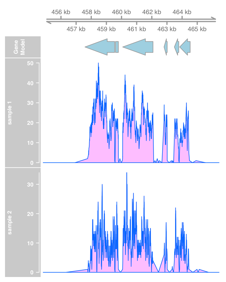
We will briefly show two packages for visualizing genomic data in Bioconductor. Note that each of these have extensive vignettes for plotting many kinds of data. We will show here how to make the coverage plots as before:

#biocLite("Gviz")
library(Gviz)
#You set up a Genome Axis Track
gtrack <- GenomeAxisTrack()
#specify an Annotation Track
atrack <- AnnotationTrack(gene, name = "Gene Model")
plotTracks(list(gtrack, atrack))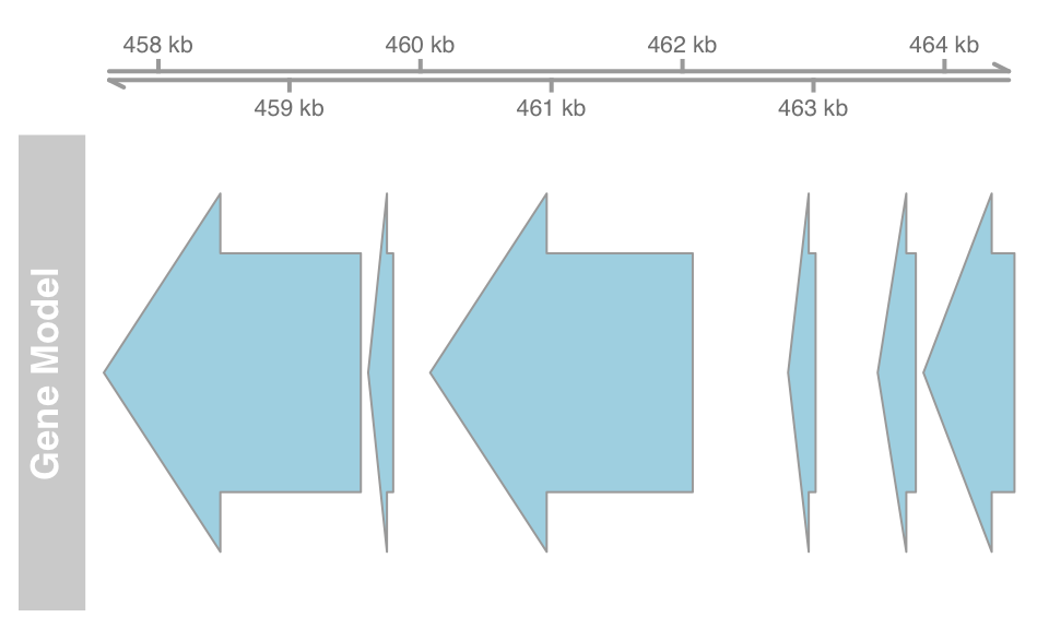

The GVIZ package also allows you to draw data. We can look at the coverage, for instance. We have the coverage already as an RleList. In order to plot coverage using the GVIZ package, you need to turn the data into a GRanges object.

Gviz expects that data will be provided as GRanges objects, so we convert the RleList coverage to a GRanges object:

#Convert coverage to GRanges object
xgr <- as(xcov, "GRanges")
ygr <- as(ycov, "GRanges")
#So we have zero coverage for the first four chromosomes, and then it says,
#chromosome four starts out with 891 base pairs of zero coverage.
#And that was the same information that we had here, 891 base pairs of zero coverage.
xgr

## GRanges with 122068 ranges and 1 metadata column:
##            seqnames              ranges strand   |     score
##                               | 
##        [1]    chr2L       [1, 23011544]      *   |         0
##        [2]    chr2R       [1, 21146708]      *   |         0
##        [3]    chr3L       [1, 24543557]      *   |         0
##        [4]    chr3R       [1, 27905053]      *   |         0
##        [5]     chr4       [1,      891]      *   |         0
##        ...      ...                 ...    ... ...       ...
##   [122064]     chr4 [1350124,  1350198]      *   |         1
##   [122065]     chr4 [1350199,  1351857]      *   |         0
##   [122066]     chrM [      1,    19517]      *   |         0
##   [122067]     chrX [      1, 22422827]      *   |         0
##   [122068]  chrYHet [      1,   347038]      *   |         0
##   ---
##   seqlengths:
##       chr2L    chr2R    chr3L    chr3R     chr4     chrM     chrX  chrYHet
##    23011544 21146708 24543557 27905053  1351857    19517 22422827   347038

#create two datatracks
#plot coverage which overlap z
dtrack1 <- DataTrack(xgr[xgr %over% z], name = "sample 1")
dtrack2 <- DataTrack(ygr[ygr %over% z], name = "sample 2")
plotTracks(list(gtrack, atrack, dtrack1, dtrack2))
plotTracks(list(gtrack, atrack, dtrack1, dtrack2), type="polygon")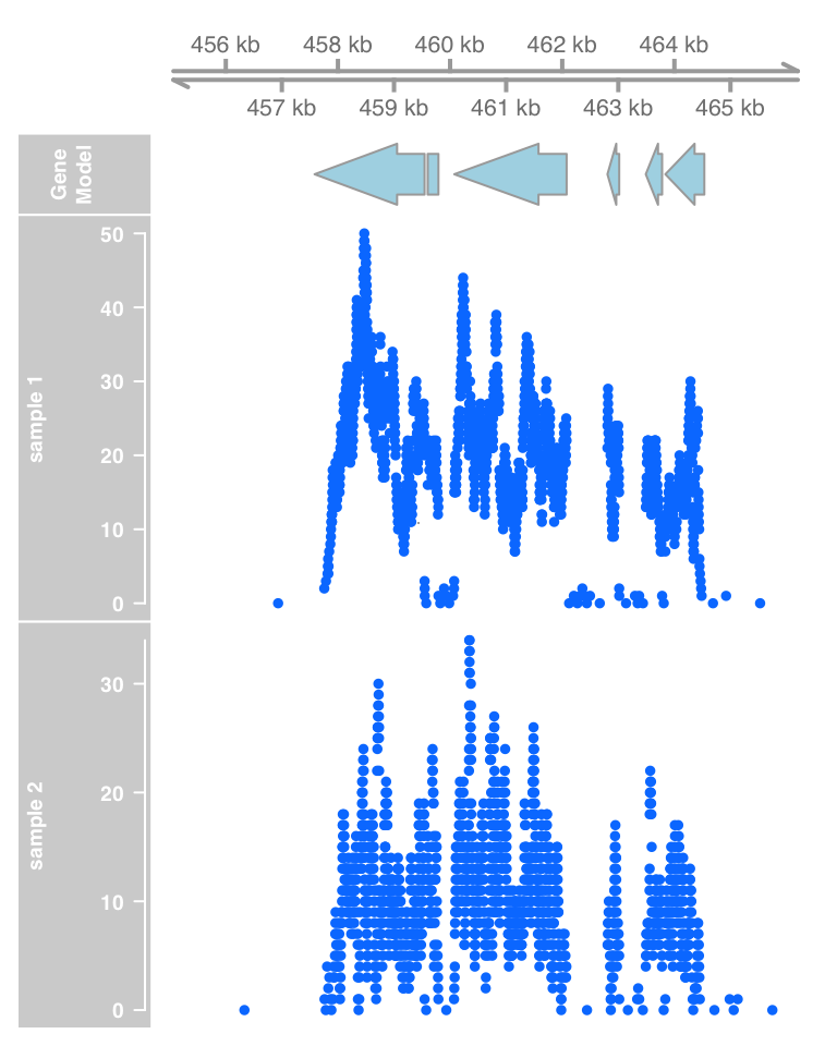

ggbio

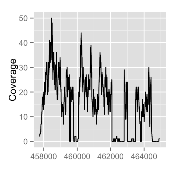
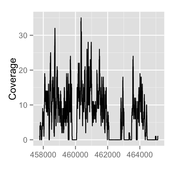
GGBIO builds off of the GGPLOT2 package, which is a whole other way of drawing plots in R. ggbio makes thing very easy. If you indicate the BAM file and the range of interest, it will read in the BAM file, parse the coverage, read the alignments, extract the information, and draw this nice plot.

#biocLite("ggbio")
library(ggbio)
#autoplot gene model
autoplot(gene)
autoplot(fl1, which=z)
autoplot(fl2, which=z)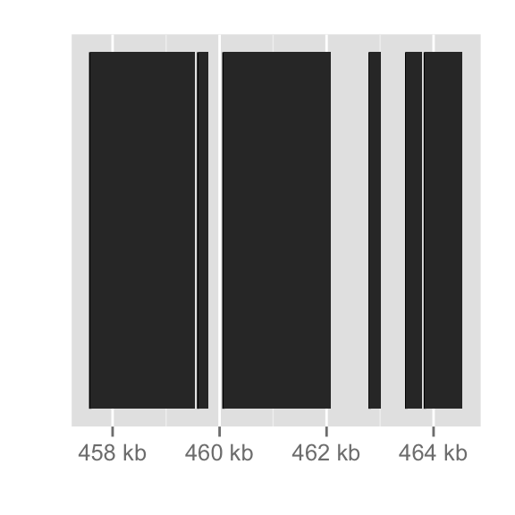

Footnotes

• IGV https://www.broadinstitute.org/igv/home

• Gviz http://www.bioconductor.org/packages/release/bioc/html/Gviz.html

• ggbio http://www.bioconductor.org/packages/release/bioc/html/ggbio.html

• UCSC Genome Browser: zooms and scrolls over chromosomes, showing the work of annotators worldwide http://genome.ucsc.edu/

• Ensembl genome browser: genome databases for vertebrates and other eukaryotic species http://ensembl.org

• Roadmap Epigenome browser: public resource of human epigenomic data http://www.epigenomebrowser.org http://genomebrowser.wustl.edu/ http://epigenomegateway.wustl.edu/

• Circos: designed for visualizing genomic data in a cirlce http://circos.ca/

• SeqMonk: a tool to visualise and analyse high throughput mapped sequence data http://www.bioinformatics.babraham.ac.uk/projects/seqmonk/

Licence

Licence

References

https://github.com/genomicsclass

Recommended for you