RNA sequencing data analysis - Counting, normalization and differential expression
This analysis was performed using R (ver. 3.1.0).
Introduction
RNA-Seq is a valuable experiment for quantifying both the types and the amount of RNA molecules in a sample.
In this article, we will focus on comparing the expression levels of different samples, by counting the number of reads which overlap the exons of genes defined by a known annotation.
Counting reads in genes
We will work with a count matrix, which has genes along the rows and samples along the columns. The elements in the matrix give the number of reads which could be uniquely aligned to a given gene for a given sample.
Load data
We will work with the Hammer et al dataset, as prepared by the ReCount website
ReCount is an online resource consisting of RNA-seq gene count datasets built using the raw data from 18 different studies. The raw sequencing data (.fastq files) were processed with Myrna to obtain tables of counts for each gene.
This is really helpful for us, so we don’t have to download all the FASTQ files and map them ourselves. If you use this resource, you should cite Frazee (2011), and cite the appropriate paper for the experimental data that you download.
Here we read in the Eset hosted by ReCount, and turn it into a SummarizedExperiment. The matrix is an expression set.
#download data
link <- "http://bowtie-bio.sourceforge.net/recount/ExpressionSets/hammer_eset.RData"
if (!file.exists("hammer_eset.RData")) download.file(link, "hammer_eset.RData")
#Load the matrix
load("hammer_eset.RData")
library(Biobase)
library(GenomicRanges)
# the SimpleList() part below is only necessary for Bioc <= 2.13
#se <- SummarizedExperiment(SimpleList(counts=exprs(hammer.eset)))
se <- SummarizedExperiment(exprs(hammer.eset))
colData(se) <- DataFrame(pData(hammer.eset))
Column data contains some informations about sample caracteristics. We have the eight samples (4 controls and four of which had spinal nerve ligation). There’s sequencing after two months after spinal nerve ligation and sequencing after two weeks of spinal nerve ligation.
#column data
colData(se)
## DataFrame with 8 rows and 5 columns
## sample.id num.tech.reps protocol strain Time
##
## SRX020102 SRX020102 1 control Sprague Dawley 2 months
## SRX020103 SRX020103 2 control Sprague Dawley 2 months
## SRX020104 SRX020104 1 L5 SNL Sprague Dawley 2 months
## SRX020105 SRX020105 2 L5 SNL Sprague Dawley 2months
## SRX020091-3 SRX020091-3 1 control Sprague Dawley 2 weeks
## SRX020088-90 SRX020088-90 2 control Sprague Dawley 2 weeks
## SRX020094-7 SRX020094-7 1 L5 SNL Sprague Dawley 2 weeks
## SRX020098-101 SRX020098-101 2 L5 SNL Sprague Dawley 2 weeks #We need to fix a typo in the Time column:
colData(se)$Time[4] <- "2 months"
colData(se)$Time <- factor(colData(se)$Time)
colData(se)$Time## [1] 2 months 2 months 2 months 2 months 2 weeks 2 weeks 2 weeks 2 weeks
## Levels: 2 months 2 weeksNormalization
Why RNAseq data should be normalized ?
The counts of the summarized experiment are in the assay slot.
#The count of experiment
head(assay(se))
## SRX020102 SRX020103 SRX020104 SRX020105 SRX020091-3 SRX020088-90 SRX020094-7 SRX020098-101
## ENSRNOG00000000001 2 4 18 24 7 4 93 77
## ENSRNOG00000000007 4 1 3 1 5 4 9 4
## ENSRNOG00000000008 0 1 4 2 0 5 2 6
## ENSRNOG00000000009 0 0 0 0 0 0 0 0
## ENSRNOG00000000010 19 10 19 13 50 57 45 58
## ENSRNOG00000000012 7 5 1 0 31 26 12 9#column sums of the count
colSums(assay(se))## SRX020102 SRX020103 SRX020104 SRX020105 SRX020091-3 SRX020088-90 SRX020094-7 SRX020098-101
## 5282855 4562100 4897807 5123782 17705411 17449646 23649094 23537179If you look at the column sums of the counts, you can see that each sample had a different amount of reads which could be aligned to the different genes. So if we’re going to do some analysis, we definitely need to take care of the fact that the different samples had different sequencing depth.
It’s not a great idea to use the number of reads which map to genes as a normalizing factor. There have been a number of papers showing that, this number is susceptible to being altered by a single gene. You might have one or a dozen genes which have very high gene expression, and those genes play the largest role in determining this sum. There are a number of more robust estimators. Probably using any of those robust estimators is better than using this sum.
We’re going to use the median ratio method, which is in the DESeq2 package.
Normalization using DESeq2 (size factors)
We will use the DESeq2 package to normalize the sample for sequencing depth. For now, don’t worry about the design argument.
In order to use this normalization method, we have to build a DESeqDataSet, which just a summarized experiment with something called a design (a formula which specifies the design of the experiment). So we’ll explain this in the next unit, but we just need to specify something. So I’m going to specify tilde 1.
# biocLite("DESeq2")
library(DESeq2)
dds <- DESeqDataSet( se, design = ~ 1 )
#names(assays(dds))
The following code estimates size factors to account for differences in sequencing depth. So the value are typically centered around 1. If all the samples have exactly the same sequencing depth, you expect these numbers to be near 1. But instead, we see that the first sample and the 7th sample have about a difference of more than 4.
#Estimate size factors
dds <- estimateSizeFactors( dds )
sizeFactors(dds)
## SRX020102 SRX020103 SRX020104 SRX020105 SRX020091-3 SRX020088-90 SRX020094-7 SRX020098-101
## 0.5211 0.4479 0.5122 0.5323 1.6893 1.6874 2.4138 2.3777colSums(counts(dds))## SRX020102 SRX020103 SRX020104 SRX020105 SRX020091-3 SRX020088-90 SRX020094-7 SRX020098-101
## 5282855 4562100 4897807 5123782 17705411 17449646 23649094 23537179#Plot column sums according to size factor
plot(sizeFactors(dds), colSums(counts(dds)))
abline(lm(colSums(counts(dds)) ~ sizeFactors(dds) + 0))
Now we can divide the columns by the size factor and take the log2 of these normalized counts plus a pseudocount of 1. We transpose in order to run PCA.
#The argument normalized equals true, divides each column by its size factor.
logcounts <- log2( counts(dds, normalized=TRUE) + 1 )
pc <- prcomp( t( logcounts ) )
Exploratory data analysis
You can see that the samples are basically clustering by the first principal component, which is in this case the protocol. More variance explained by protocol than by time. You could also do a hierarchical clustering, and you could see that here again, they’re separated more by protocol than by time. You can see they don’t actually cluster discreetly by time.
#library(devtools)
#install_github("rafalib", "ririzarr")
library(rafalib)
#PC 1 VS PC 2
plot(pc$x[,1], pc$x[,2],
     col=colData(dds)$protocol, # color is the protocol
     pch=as.numeric(colData(dds)$Time)+15)# point shape by time
#hierarchical clustering
plot(hclust(dist(t(logcounts))), labels=colData(dds)$protocol)
plot(hclust(dist(t(logcounts))), labels=colData(dds)$Time)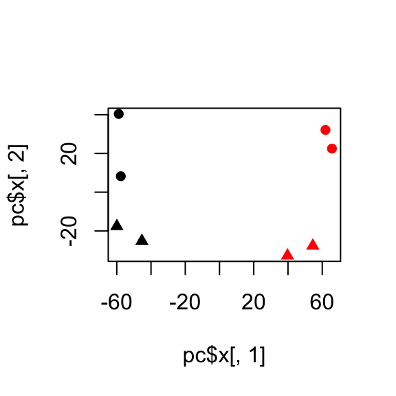


And finally, we can just take a look at the log accounts of the first two samples against each other. What I’m trying to point out here is, as we saw in an earlier unit, you can see there’s a spread of the points. So there’s extra variance in the log space when you get down to low values, which is sometimes called Poisson noise.
#log count of the first two samples
plot(logcounts[,1], logcounts[,2], cex=.1)
Now we will use a normalization method, which is similar to the variance stablizing normalization method mentioned. It uses the variance model to shrink together the sample values for lowly expressed genes with high variance.
Normalization to stabilize variance (regularized logarithm)
The data is in the assay slot, and needs to be transposed as before to run PCA.
# this takes ~15 seconds
# normalization to stabilize variance (regularized logarithm)
rld <- rlog( dds ) # object of class GenomicRanges
# if using Bioc 2.13:
# rld <- rlogTransformation( dds )
We see again, the protocol drives the variance. But if you look at the time dimension, now the times cluster together discreetly. So instead of before, we had two months joining with the two weeks, now they join each other first, and then they join as a protocol. We could look at the plot of the first sample against the second sample. We can see what, the values near 0 were shrunk towards each other.
We can look at the same plots now using this transformed data:
pc2 <- prcomp( t( assay(rld) ) )
plot(pc2$x[,1], pc2$x[,2],  col=colData(rld)$protocol,pch=as.numeric(colData(rld)$Time)+15)
plot(hclust(dist(t(assay(rld)))), labels=colData(rld)$protocol)
plot(hclust(dist(t(assay(rld)))), labels=colData(rld)$Time)
plot(assay(rld)[,1], assay(rld)[,2], cex=.1)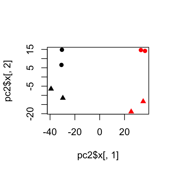


Differential gene expression
A number of methods for assessing differential gene expression from RNA-Seq counts use the Negative Binomial distribution to make probabilistic statements about the differences seen in an experiment. A few such methods are edgeR, DESeq, DSS and many others. A very incomplete list of other methods is provided in the footnotes.
We will use DESeq2 to perform differential gene expression on the counts. This also uses a Negative Binomial distribution to model the counts. It performs a similar step to limma, in using the variance of all the genes to improve the variance estimate for each individual gene. In addition, it shrinks the high variance fold changes, which will be seen in the resulting MA-plot.
Before we specified a design for this, which was just tilde 1. And that represented just modeling these counts on an intercept value. But for differential expression analysis, we want to model them based on the design of the experiment. The design of the experiment was two different treatments, spinal nerve ligation and control, and sequencing was done at two different times.
First, we setup the design of the experiment, so that differences will be considered across time and protocol variables. The last variable is used for the default results tables and plots, and we make sure the “control” level is the first level, such that log fold changes will be treatment over control, and not control over treatment.
If control was not the base level, because the factoring is done alphabetically, you could use the relevel function in R, and give it the level that you want to be the first. So this would just then set control as the first level, if it wasn’t already so.
colData(dds)$protocol## [1] control control L5 SNL L5 SNL control control L5 SNL L5 SNL
## Levels: control L5 SNL# if control was not already the "base level", we would do:
# set control as the first level, if it wasn't already so.
colData(dds)$protocol <- relevel(colData(dds)$protocol, "control")
levels(colData(dds)$protocol)## [1] "control" "L5 SNL"#Change the design
design(dds) <- ~ Time + protocolWe put the protocol as the last variable of the design, because this is the variable that will be used to generate log fold changes. So we want to know, controlling for time, what genes were changed according to the protocol.
The following line runs the model, and then we can extract a results table for all genes:
# this takes ~20 seconds
dds <- DESeq( dds )
res <- results( dds )
head(res)
## log2 fold change (MAP): protocol L5 SNL vs control
## Wald test p-value: protocol L5 SNL vs control
## DataFrame with 6 rows and 6 columns
## baseMean log2FoldChange lfcSE stat pvalue padj
##
## ENSRNOG00000000001 21.304 2.9267 0.4055 7.2180 5.275e-13 4.219e-12
## ENSRNOG00000000007 3.548 -0.1309 0.6373 -0.2054 8.373e-01 8.886e-01
## ENSRNOG00000000008 2.514 0.7699 0.7314 1.0526 2.925e-01 4.039e-01
## ENSRNOG00000000009 0.000 NA NA NA NA NA
## ENSRNOG00000000010 28.340 -0.3193 0.2899 -1.1013 2.708e-01 3.798e-01
## ENSRNOG00000000012 8.633 -1.9587 0.4943 -3.9628 7.409e-05 2.411e-04 baseMean is the average mean expression stat = log2FoldChange/ lfcSE
We can also make other results tables, such as control over SNL, or for comparing the time variable.
#switch the numerator and the denominator
#For the protocol variable I want the control over L5 SNL
head(results(dds, contrast=c("protocol","control","L5 SNL")))
## log2 fold change (MAP): protocol control vs L5 SNL
## Wald test p-value: protocol control vs L5 SNL
## DataFrame with 6 rows and 6 columns
## baseMean log2FoldChange lfcSE stat pvalue padj
##
## ENSRNOG00000000001 21.304 -2.9267 0.4055 -7.2180 5.275e-13 4.219e-12
## ENSRNOG00000000007 3.548 0.1309 0.6373 0.2054 8.373e-01 8.886e-01
## ENSRNOG00000000008 2.514 -0.7699 0.7314 -1.0526 2.925e-01 4.039e-01
## ENSRNOG00000000009 0.000 NA NA NA NA NA
## ENSRNOG00000000010 28.340 0.3193 0.2899 1.1013 2.708e-01 3.798e-01
## ENSRNOG00000000012 8.633 1.9587 0.4943 3.9628 7.409e-05 2.411e-04 #You can also build result for time variable
head(results(dds, contrast=c("Time","2 months","2 weeks")))## log2 fold change (MAP): Time 2 months vs 2 weeks
## Wald test p-value: Time 2 months vs 2 weeks
## DataFrame with 6 rows and 6 columns
## baseMean log2FoldChange lfcSE stat pvalue padj
##
## ENSRNOG00000000001 21.304 0.2950 0.3227 0.9143 0.3605 0.5496
## ENSRNOG00000000007 3.548 0.3728 0.4307 0.8656 0.3867 NA
## ENSRNOG00000000008 2.514 0.3814 0.4162 0.9163 0.3595 NA
## ENSRNOG00000000009 0.000 NA NA NA NA NA
## ENSRNOG00000000010 28.340 0.1863 0.2753 0.6766 0.4986 0.6726
## ENSRNOG00000000012 8.633 -0.5253 0.4018 -1.3073 0.1911 NA We can now contruct an MA-plot of the fold change over the average expression level of all samples.
# Bioc 2.13
plotMA(dds, ylim=c(-5,5))
# Bioc 2.14
plotMA(res, ylim=c(-5,5))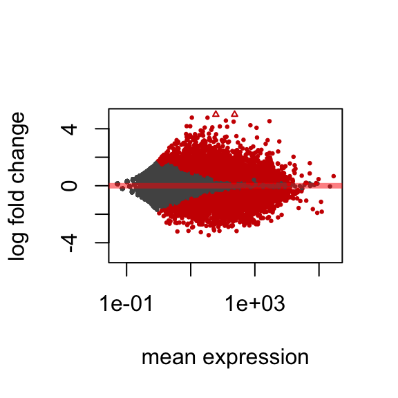
And you can see, highlighted in red, are those genes which had an adjusted p-value less than 0.1.
Suppose we are not interested in small log2 fold changes even if they are significantly differentially expressed. We can also test for log2 fold changes larger than 1 in absolute value.
So there’s a way to specify this to the results function, to say I’m only interested in genes which have a log 2 fold change greater in absolute value than 1. And this is not just filtering based on the fold change, but it’s actually performing a statistical test.
resBigFC <- results(dds, lfcThreshold=1, altHypothesis="greaterAbs")
plotMA(resBigFC, ylim=c(-5,5))
abline(h=c(-1,1),lwd=5)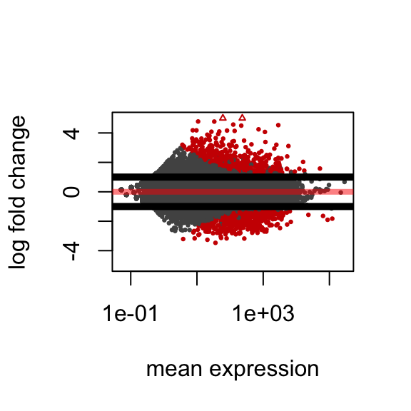
Let’s examine the top gene, sorting by p-value:
#Top genes : sort by pvalue
resSort <- res[order(res$pvalue),]
head(resSort)
## log2 fold change (MAP): protocol L5 SNL vs control
## Wald test p-value: protocol L5 SNL vs control
## DataFrame with 6 rows and 6 columns
## baseMean log2FoldChange lfcSE stat pvalue padj
##
## ENSRNOG00000004805 1127.9 4.068 0.10665 38.15 0.000e+00 0.000e+00
## ENSRNOG00000004874 1271.5 2.498 0.08466 29.50 2.532e-191 2.016e-187
## ENSRNOG00000015156 1166.1 3.383 0.12076 28.01 1.090e-172 5.784e-169
## ENSRNOG00000004731 892.4 -2.588 0.09352 -27.67 1.620e-168 6.450e-165
## ENSRNOG00000003745 2495.9 3.196 0.12372 25.83 3.707e-147 1.181e-143
## ENSRNOG00000032884 3219.1 -2.466 0.09607 -25.66 2.889e-145 7.669e-142 #Count for the first gene: the unnormalized count
k <- counts(dds)[rownames(resSort)[1],]
#Make a stripchart by combining time and protocol
cond <- with(colData(se), factor(paste(Time, protocol)))
stripchart(log2(k + 1) ~ cond, method="jitter", vertical=TRUE, las=2)
You can see why this was given such a low p-value is because if you look at this change from control to spinal nerve ligation, it’s a very large log2 fold change. And it’s consistent, also, across time. And that leads to this very low p-value.
We can then check the annotation of these highly significant genes:
# biocLite("org.Rn.eg.db")
library(org.Rn.eg.db)
#The keys we can query on Ensembl
keytypes(org.Rn.eg.db)
## [1] "ENTREZID" "PFAM" "IPI" "PROSITE" "ACCNUM" "ALIAS" "CHR"
## [8] "CHRLOC" "CHRLOCEND" "ENZYME" "PATH" "PMID" "REFSEQ" "SYMBOL"
## [15] "UNIGENE" "ENSEMBL" "ENSEMBLPROT" "ENSEMBLTRANS" "GENENAME" "UNIPROT" "GO"
## [22] "EVIDENCE" "ONTOLOGY" "GOALL" "EVIDENCEALL" "ONTOLOGYALL"head(rownames(dds))## [1] "ENSRNOG00000000001" "ENSRNOG00000000007" "ENSRNOG00000000008" "ENSRNOG00000000009" "ENSRNOG00000000010"
## [6] "ENSRNOG00000000012"#The first 20 genes according to the lowest p-value
geneinfo <- select(org.Rn.eg.db, keys=rownames(resSort)[1:20],
columns=c("ENSEMBL","SYMBOL","GENENAME"),
keytype="ENSEMBL")
geneinfo## ENSEMBL SYMBOL GENENAME
## 1 ENSRNOG00000004805 Stac2 SH3 and cysteine rich domain 2
## 2 ENSRNOG00000004874 Flrt3 fibronectin leucine rich transmembrane protein 3
## 3 ENSRNOG00000015156 Gal galanin/GMAP prepropeptide
## 4 ENSRNOG00000004731 Ano3 anoctamin 3
## 5 ENSRNOG00000003745 Atf3 activating transcription factor 3
## 6 ENSRNOG00000032884 Scn11a sodium channel, voltage-gated, type XI, alpha subunit
## 7 ENSRNOG00000018808 Vip vasoactive intestinal peptide
## 8 ENSRNOG00000033531 Cacna2d1 calcium channel, voltage-dependent, alpha2/delta subunit 1
## 9 ENSRNOG00000032473 Scn10a sodium channel, voltage-gated, type X, alpha subunit
## 10 ENSRNOG00000019486 Trpv1 transient receptor potential cation channel, subfamily V, member 1
## 11 ENSRNOG00000009186 Stmn4 stathmin-like 4
## 12 ENSRNOG00000012448 Chrnb3 cholinergic receptor, nicotinic, beta 3 (neuronal)
## 13 ENSRNOG00000019574 Cuedc2 CUE domain containing 2
## 14 ENSRNOG00000031997
## 15 ENSRNOG00000002595 Dpp10 dipeptidylpeptidase 10
## 16 ENSRNOG00000027331 Ppef1 protein phosphatase, EF-hand calcium binding domain 1
## 17 ENSRNOG00000015055 Scg2 secretogranin II
## 18 ENSRNOG00000000129 RGD1559864 similar to mKIAA1045 protein
## 19 ENSRNOG00000003386 Rbfox3 RNA binding protein, fox-1 homolog (C. elegans) 3
## 20 ENSRNOG00000020136 Tgm1 transglutaminase 1 Footnotes
Introduction
Mortazavi A, Williams BA, McCue K, Schaeffer L, Wold B., “Mapping and quantifying mammalian transcriptomes by RNA-Seq”, Nat Methods. 2008. http://www.nature.com/nmeth/journal/v5/n7/full/nmeth.1226.html
John C. Marioni, Christopher E. Mason, Shrikant M. Mane, Matthew Stephens, and Yoav Gilad, “RNA-seq: An assessment of technical reproducibility and comparison with gene expression arrays” Genome Res. 2008. http://www.ncbi.nlm.nih.gov/pmc/articles/PMC2527709/
Hammer et al
Hammer P, Banck MS, Amberg R, Wang C, Petznick G, Luo S, Khrebtukova I, Schroth GP, Beyerlein P, Beutler AS. “mRNA-seq with agnostic splice site discovery for nervous system transcriptomics tested in chronic pain.” Genome Res. 2010 http://www.ncbi.nlm.nih.gov/pubmed?term=20452967
ReCount
Frazee AC, Langmead B, Leek JT. “ReCount: a multi-experiment resource of analysis-ready RNA-seq gene count datasets”. BMC Bioinformatics 12:449 http://www.ncbi.nlm.nih.gov/pubmed/22087737
Negative Binomial methods for differential expression of count data
All the following methods are available on Bioconductor:
edgeR
Mark D. Robinson, Davis J. McCarthy, and Gordon K. Smyth, “edgeR: a Bioconductor package for differential expression analysis of digital gene expression data” Bioinformatics 2010. http://www.ncbi.nlm.nih.gov/pmc/articles/PMC2796818/
DESeq(the latest version is a separate package,DESeq2)
Simon Anders and Wolfgang Huber, “Differential expression analysis for sequence count data”, Genome Biology 2010. http://genomebiology.com/2010/11/10/r106
DSS
Hao Wu, Chi Wang, Zhijin Wu, “A new shrinkage estimator for dispersion improves differential expression detection in RNA-seq data” Biostatistics 2013. http://biostatistics.oxfordjournals.org/content/14/2/232
Transformation followed by linear model methods
voom in the limma Bioconductor package
Charity W Law, Yunshun Chen, Wei Shi and Gordon K Smyth, “voom: precision weights unlock linear model analysis tools for RNA-seq read counts”, Genome Biology. 2014. http://genomebiology.com/2014/15/2/R29
Resampling-based methods
SAMseq in the samr package on CRAN
Jun Li and Robert Tibshirani, “Finding consistent patterns: A nonparametric approach for identifying differential expression in RNA-Seq data”, Stat Methods Med Res. 2013. http://smm.sagepub.com/content/22/5/519.short
Incorporating isoform-abundance
Cuffdiff(the latest version isCuffdiff2)
Trapnell C, Hendrickson DG, Sauvageau M, Goff L, Rinn JL, Pachter L., “Differential analysis of gene regulation at transcript resolution with RNA-seq” Nat Biotechnol. 2013. http://www.ncbi.nlm.nih.gov/pubmed/23222703
BitSeq
Peter Glaus, Antti Honkela, and Magnus Rattray, “Identifying differentially expressed transcripts from RNA-seq data with biological variation”, Bioinformatics. 2012. http://bioinformatics.oxfordjournals.org/content/28/13/1721
Licence
References
Show me some love with the like buttons below... Thank you and please don't forget to share and comment below!!
Montrez-moi un peu d'amour avec les like ci-dessous ... Merci et n'oubliez pas, s'il vous plaît, de partager et de commenter ci-dessous!
Recommended for You!
Recommended for you
This section contains the best data science and self-development resources to help you on your path.
Books - Data Science
Our Books
- Practical Guide to Cluster Analysis in R by A. Kassambara (Datanovia)
- Practical Guide To Principal Component Methods in R by A. Kassambara (Datanovia)
- Machine Learning Essentials: Practical Guide in R by A. Kassambara (Datanovia)
- R Graphics Essentials for Great Data Visualization by A. Kassambara (Datanovia)
- GGPlot2 Essentials for Great Data Visualization in R by A. Kassambara (Datanovia)
- Network Analysis and Visualization in R by A. Kassambara (Datanovia)
- Practical Statistics in R for Comparing Groups: Numerical Variables by A. Kassambara (Datanovia)
- Inter-Rater Reliability Essentials: Practical Guide in R by A. Kassambara (Datanovia)
Others
- R for Data Science: Import, Tidy, Transform, Visualize, and Model Data by Hadley Wickham & Garrett Grolemund
- Hands-On Machine Learning with Scikit-Learn, Keras, and TensorFlow: Concepts, Tools, and Techniques to Build Intelligent Systems by Aurelien Géron
- Practical Statistics for Data Scientists: 50 Essential Concepts by Peter Bruce & Andrew Bruce
- Hands-On Programming with R: Write Your Own Functions And Simulations by Garrett Grolemund & Hadley Wickham
- An Introduction to Statistical Learning: with Applications in R by Gareth James et al.
- Deep Learning with R by François Chollet & J.J. Allaire
- Deep Learning with Python by François Chollet
Click to follow us on Facebook :
Comment this article by clicking on "Discussion" button (top-right position of this page)


