


ggplot2 texts : Add text annotations to a graph in R software
- Install required packages
- Create some data
- Text annotations using geom_text and geom_label
- Change the text color and size by groups
- Add a text annotation at a particular coordinate
- annotation_custom : Add a static text annotation in the top-right, top-left, …
- ggrepel: Avoid overlapping of text labels
- Infos
This article describes how to add a text annotation to a plot generated using ggplot2 package.
The functions below can be used :
- geom_text(): adds text directly to the plot
- geom_label(): draws a rectangle underneath the text, making it easier to read.
- annotate(): useful for adding small text annotations at a particular location on the plot
- annotation_custom(): Adds static annotations that are the same in every panel
It’s also possible to use the R package ggrepel, which is an extension and provides geom for ggplot2 to repel overlapping text labels away from each other.
We’ll start by describing how to use ggplot2 official functions for adding text annotations. In the last sections, examples using ggrepel extensions are provided.
Related Book:
GGPlot2 Essentials for Great Data Visualization in R
Install required packages
# Install ggplot2
install.packages("ggplot2")
# Install ggrepel
install.packages("ggrepel")
Create some data
We’ll use a subset of mtcars data. The function sample() can be used to randomly extract 10 rows:
# Subset 10 rows
set.seed(1234)
ss <- sample(1:32, 10)
df <- mtcars[ss, ]
Text annotations using geom_text and geom_label
library(ggplot2)
# Simple scatter plot
sp <- ggplot(df, aes(wt, mpg, label = rownames(df)))+
geom_point()
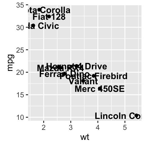
# Add texts
sp + geom_text()
# Change the size of the texts
sp + geom_text(size=6)
# Change vertical and horizontal adjustement
sp + geom_text(hjust=0, vjust=0)
# Change fontface. Allowed values : 1(normal),
# 2(bold), 3(italic), 4(bold.italic)
sp + geom_text(aes(fontface=2))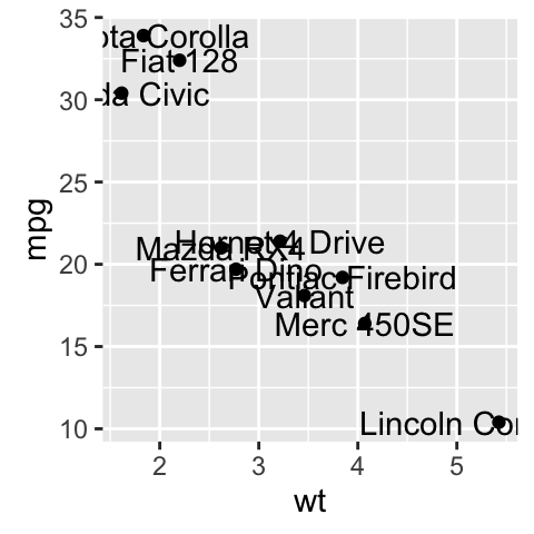
- Change font family
sp + geom_text(family = "Times New Roman")- geom_label() works like geom_text() but draws a rounded rectangle underneath each label. This is useful when you want to label plots that are dense with data.
sp + geom_label()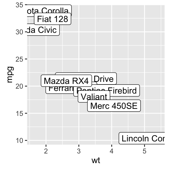
Others useful arguments for geom_text() and geom_label() are:
- nudge_x and nudge_y: let you offset labels from their corresponding points. The function position_nudge() can be also used.
- check_overlap = TRUE: for avoiding overplotting of labels
- hjust and vjust can now be character vectors (ggplot2 v >= 2.0.0): “left”, “center”, “right”, “bottom”, “middle”, “top”. New options include “inward” and “outward” which align text towards and away from the center of the plot respectively.
Change the text color and size by groups
It’s possible to change the appearance of the texts using aesthetics (color, size,…) :
sp2 <- ggplot(mtcars, aes(x=wt, y=mpg, label=rownames(mtcars)))+
  geom_point()
# Color by groups
sp2 + geom_text(aes(color=factor(cyl)))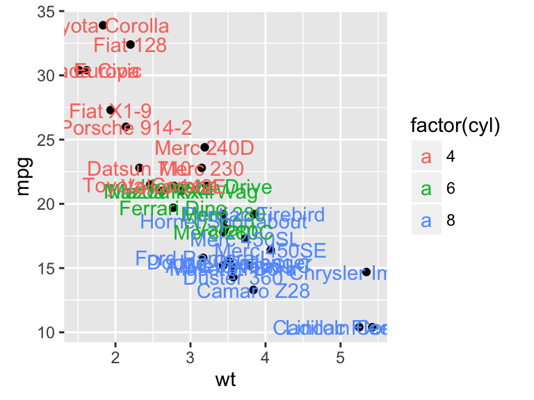
# Set the size of the text using a continuous variable
sp2 + geom_text(aes(size=wt))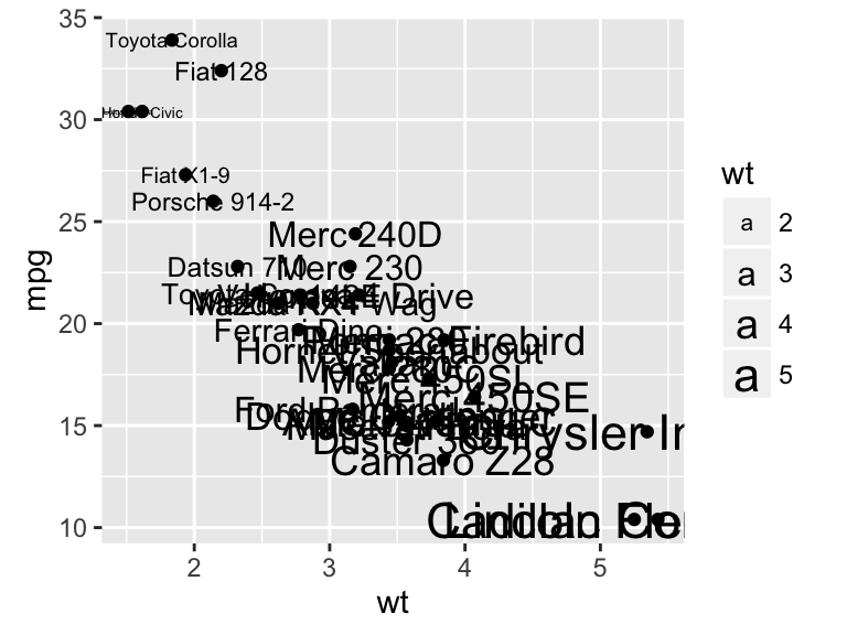
# Define size range
sp2 + geom_text(aes(size=wt)) + scale_size(range=c(3,6))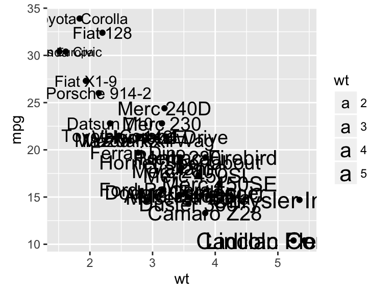
Add a text annotation at a particular coordinate
The functions geom_text() and annotate() can be used :
# Solution 1
sp2 + geom_text(x=3, y=30, label="Scatter plot")
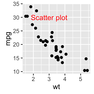
# Solution 2
sp2 + annotate(geom="text", x=3, y=30, label="Scatter plot",
color="red")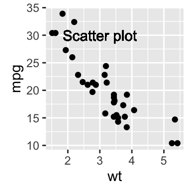
annotation_custom : Add a static text annotation in the top-right, top-left, …
The functions annotation_custom() and textGrob() are used to add static annotations which are the same in every panel.The grid package is required :
library(grid)
# Create a text
grob <- grobTree(textGrob("Scatter plot", x=0.1,  y=0.95, hjust=0,
  gp=gpar(col="red", fontsize=13, fontface="italic")))
# Plot
sp2 + annotation_custom(grob)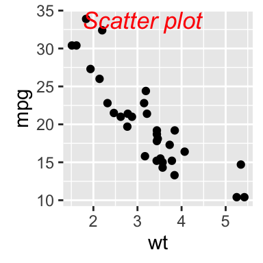
Facet : In the plot below, the annotation is at the same place (in each facet) even if the axis scales vary.
sp2 + annotation_custom(grob)+facet_wrap(~cyl, scales="free")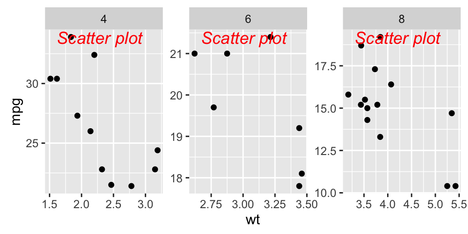
ggrepel: Avoid overlapping of text labels
There are two important functions in ggrepel R packages:
- geom_label_repel()
- geom_text_repel()
Scatter plots with text annotations
We start by creating a simple scatter plot using a subset of the mtcars data set containing 15 rows.
- Prepare some data:
# Take a subset of 15 random points
set.seed(1234)
ss <- sample(1:32, 15)
df <- mtcars[ss, ]- Create a scatter plot:
p <- ggplot(df, aes(wt, mpg)) +
  geom_point(color = 'red') +
theme_classic(base_size = 10)- Add text labels:
# Add text annotations using ggplot2::geom_text
p + geom_text(aes(label = rownames(df)),
              size = 3.5)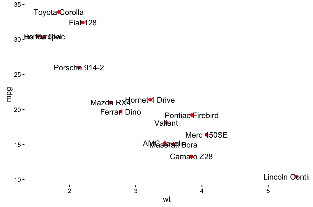
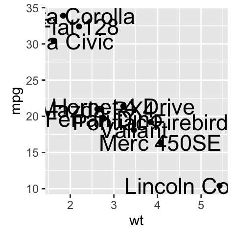
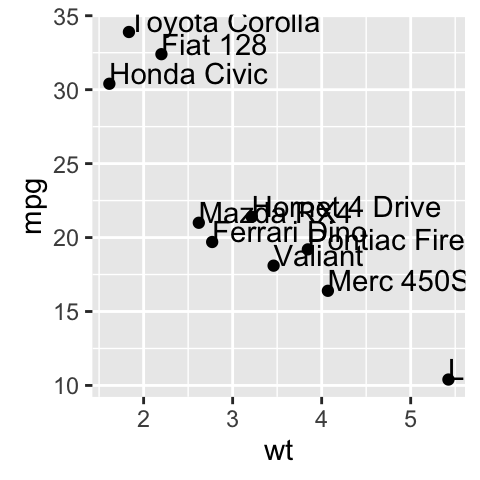
# Use ggrepel::geom_text_repel
require("ggrepel")
set.seed(42)
p + geom_text_repel(aes(label = rownames(df)),
size = 3.5) 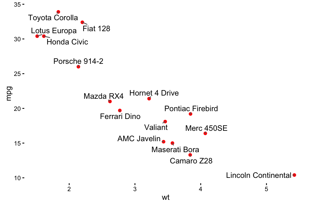
# Use ggrepel::geom_label_repel and
# Change color by groups
set.seed(42)
p + geom_label_repel(aes(label = rownames(df),
                    fill = factor(cyl)), color = 'white',
                    size = 3.5) +
   theme(legend.position = "bottom")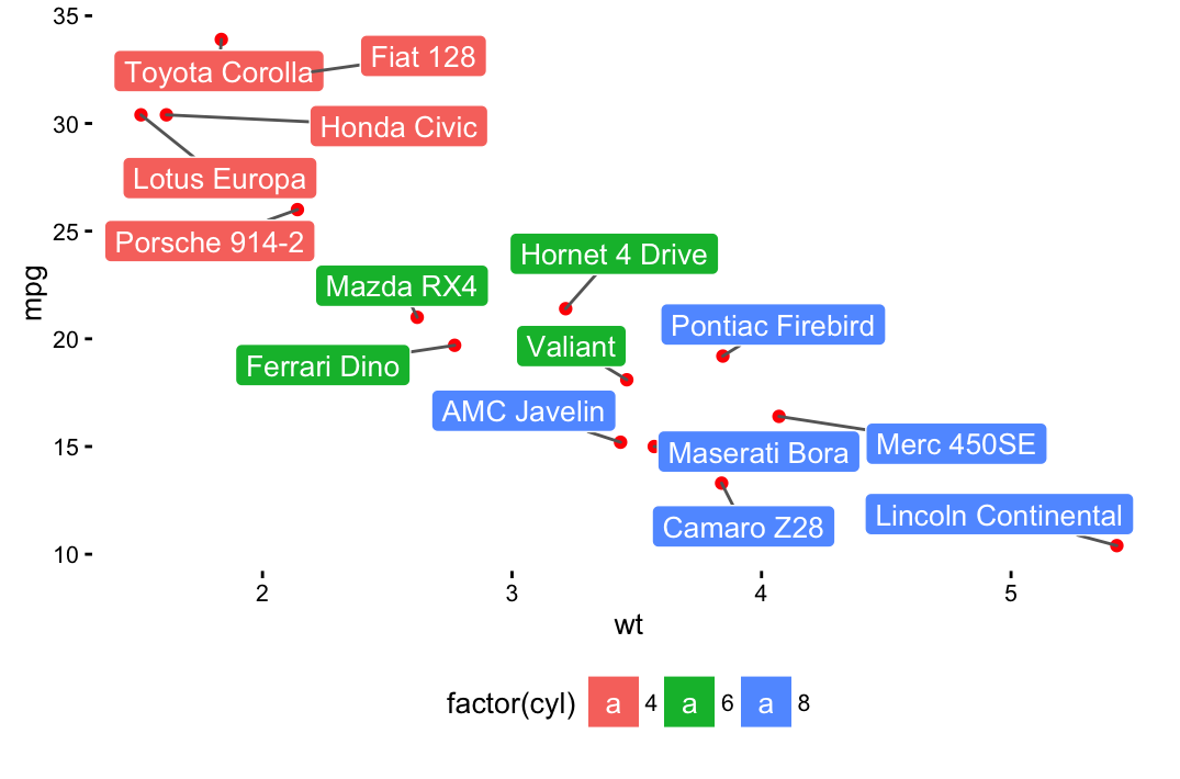
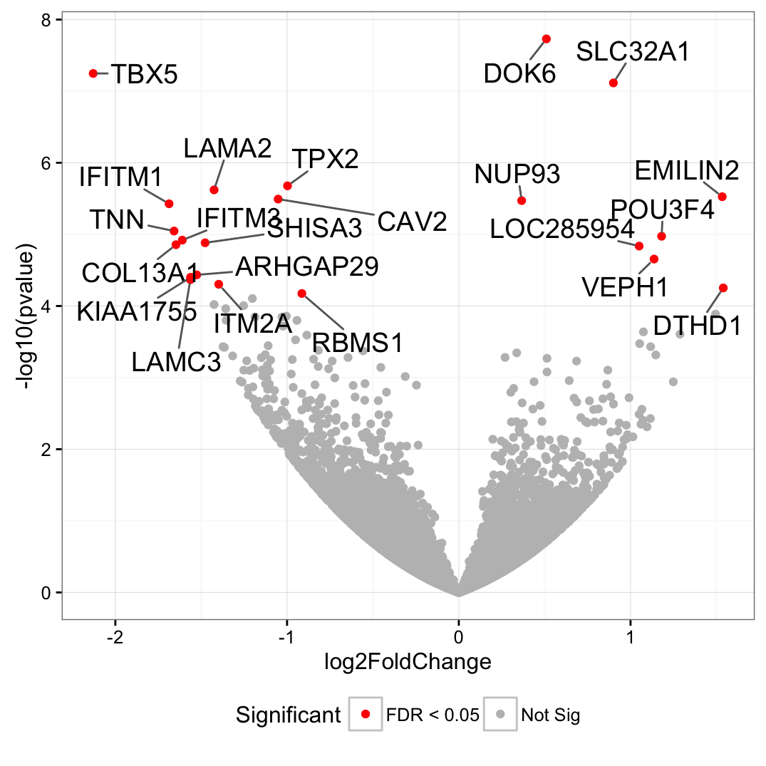
Volcano plot
genes <- read.table("https://gist.githubusercontent.com/stephenturner/806e31fce55a8b7175af/raw/1a507c4c3f9f1baaa3a69187223ff3d3050628d4/results.txt", header = TRUE)
genes$Significant <- ifelse(genes$padj < 0.05, "FDR < 0.05", "Not Sig")
ggplot(genes, aes(x = log2FoldChange, y = -log10(pvalue))) +
  geom_point(aes(color = Significant)) +
  scale_color_manual(values = c("red", "grey")) +
  theme_bw(base_size = 12) + theme(legend.position = "bottom") +
  geom_text_repel(
    data = subset(genes, padj < 0.05),
    aes(label = Gene),
    size = 5,
    box.padding = unit(0.35, "lines"),
    point.padding = unit(0.3, "lines")
  )
Infos
This analysis has been performed using R software (ver. 3.2.4) and ggplot2 (ver. )
Show me some love with the like buttons below... Thank you and please don't forget to share and comment below!!
Montrez-moi un peu d'amour avec les like ci-dessous ... Merci et n'oubliez pas, s'il vous plaît, de partager et de commenter ci-dessous!
Recommended for You!


Recommended for you
This section contains the best data science and self-development resources to help you on your path.
Books - Data Science
Our Books
- Practical Guide to Cluster Analysis in R by A. Kassambara (Datanovia)
- Practical Guide To Principal Component Methods in R by A. Kassambara (Datanovia)
- Machine Learning Essentials: Practical Guide in R by A. Kassambara (Datanovia)
- R Graphics Essentials for Great Data Visualization by A. Kassambara (Datanovia)
- GGPlot2 Essentials for Great Data Visualization in R by A. Kassambara (Datanovia)
- Network Analysis and Visualization in R by A. Kassambara (Datanovia)
- Practical Statistics in R for Comparing Groups: Numerical Variables by A. Kassambara (Datanovia)
- Inter-Rater Reliability Essentials: Practical Guide in R by A. Kassambara (Datanovia)
Others
- R for Data Science: Import, Tidy, Transform, Visualize, and Model Data by Hadley Wickham & Garrett Grolemund
- Hands-On Machine Learning with Scikit-Learn, Keras, and TensorFlow: Concepts, Tools, and Techniques to Build Intelligent Systems by Aurelien Géron
- Practical Statistics for Data Scientists: 50 Essential Concepts by Peter Bruce & Andrew Bruce
- Hands-On Programming with R: Write Your Own Functions And Simulations by Garrett Grolemund & Hadley Wickham
- An Introduction to Statistical Learning: with Applications in R by Gareth James et al.
- Deep Learning with R by François Chollet & J.J. Allaire
- Deep Learning with Python by François Chollet
Click to follow us on Facebook :
Comment this article by clicking on "Discussion" button (top-right position of this page)