


Nonlinear Regression Essentials in R: Polynomial and Spline Regression Models
In some cases, the true relationship between the outcome and a predictor variable might not be linear.
There are different solutions extending the linear regression model (Chapter @ref(linear-regression)) for capturing these nonlinear effects, including:
Polynomial regression. This is the simple approach to model non-linear relationships. It add polynomial terms or quadratic terms (square, cubes, etc) to a regression.
Spline regression. Fits a smooth curve with a series of polynomial segments. The values delimiting the spline segments are called Knots.
Generalized additive models (GAM). Fits spline models with automated selection of knots.
In this chapter, you’ll learn how to compute non-linear regression models and how to compare the different models in order to choose the one that fits the best your data.
The RMSE and the R2 metrics, will be used to compare the different models (see Chapter @ref(linear regression)).
Recall that, the RMSE represents the model prediction error, that is the average difference the observed outcome values and the predicted outcome values. The R2 represents the squared correlation between the observed and predicted outcome values. The best model is the model with the lowest RMSE and the highest R2.
Contents:

Loading Required R packages
tidyversefor easy data manipulation and visualizationcaretfor easy machine learning workflow
library(tidyverse)
library(caret)
theme_set(theme_classic())
Preparing the data
We’ll use the Boston data set [in MASS package], introduced in Chapter @ref(regression-analysis), for predicting the median house value (mdev), in Boston Suburbs, based on the predictor variable lstat (percentage of lower status of the population).
We’ll randomly split the data into training set (80% for building a predictive model) and test set (20% for evaluating the model). Make sure to set seed for reproducibility.
# Load the data
data("Boston", package = "MASS")
# Split the data into training and test set
set.seed(123)
training.samples <- Boston$medv %>%
  createDataPartition(p = 0.8, list = FALSE)
train.data  <- Boston[training.samples, ]
test.data <- Boston[-training.samples, ]
First, visualize the scatter plot of the medv vs lstat variables as follow:
ggplot(train.data, aes(lstat, medv) ) +
  geom_point() +
  stat_smooth()
The above scatter plot suggests a non-linear relationship between the two variables
In the following sections, we start by computing linear and non-linear regression models. Next, we’ll compare the different models in order to choose the best one for our data.
Linear regression {linear-reg}
The standard linear regression model equation can be written as medv = b0 + b1*lstat.
Compute linear regression model:
# Build the model
model <- lm(medv ~ lstat, data = train.data)
# Make predictions
predictions <- model %>% predict(test.data)
# Model performance
data.frame(
  RMSE = RMSE(predictions, test.data$medv),
  R2 = R2(predictions, test.data$medv)
)
## RMSE R2
## 1 6.07 0.535Visualize the data:
ggplot(train.data, aes(lstat, medv) ) +
  geom_point() +
  stat_smooth(method = lm, formula = y ~ x)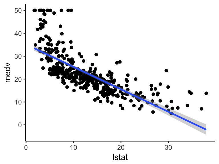
Polynomial regression
The polynomial regression adds polynomial or quadratic terms to the regression equation as follow:
\[medv = b0 + b1*lstat + b2*lstat^2\]
In R, to create a predictor x^2 you should use the function I(), as follow: I(x^2). This raise x to the power 2.
The polynomial regression can be computed in R as follow:
lm(medv ~ lstat + I(lstat^2), data = train.data)An alternative simple solution is to use this:
lm(medv ~ poly(lstat, 2, raw = TRUE), data = train.data)##
## Call:
## lm(formula = medv ~ poly(lstat, 2, raw = TRUE), data = train.data)
##
## Coefficients:
## (Intercept) poly(lstat, 2, raw = TRUE)1
## 43.351 -2.340
## poly(lstat, 2, raw = TRUE)2
## 0.043The output contains two coefficients associated with lstat : one for the linear term (lstat^1) and one for the quadratic term (lstat^2).
The following example computes a sixfth-order polynomial fit:
lm(medv ~ poly(lstat, 6, raw = TRUE), data = train.data) %>%
  summary()
##
## Call:
## lm(formula = medv ~ poly(lstat, 6, raw = TRUE), data = train.data)
##
## Residuals:
## Min 1Q Median 3Q Max
## -14.23 -3.24 -0.74 2.02 26.50
##
## Coefficients:
## Estimate Std. Error t value Pr(>|t|)
## (Intercept) 7.14e+01 6.00e+00 11.90 < 2e-16 ***
## poly(lstat, 6, raw = TRUE)1 -1.45e+01 3.22e+00 -4.48 9.6e-06 ***
## poly(lstat, 6, raw = TRUE)2 1.87e+00 6.26e-01 2.98 0.003 **
## poly(lstat, 6, raw = TRUE)3 -1.32e-01 5.73e-02 -2.30 0.022 *
## poly(lstat, 6, raw = TRUE)4 4.98e-03 2.66e-03 1.87 0.062 .
## poly(lstat, 6, raw = TRUE)5 -9.56e-05 6.03e-05 -1.58 0.114
## poly(lstat, 6, raw = TRUE)6 7.29e-07 5.30e-07 1.38 0.170
## ---
## Signif. codes: 0 '***' 0.001 '**' 0.01 '*' 0.05 '.' 0.1 ' ' 1
##
## Residual standard error: 5.28 on 400 degrees of freedom
## Multiple R-squared: 0.684, Adjusted R-squared: 0.679
## F-statistic: 144 on 6 and 400 DF, p-value: <2e-16From the output above, it can be seen that polynomial terms beyond the fith order are not significant. So, just create a fith polynomial regression model as follow:
# Build the model
model <- lm(medv ~ poly(lstat, 5, raw = TRUE), data = train.data)
# Make predictions
predictions <- model %>% predict(test.data)
# Model performance
data.frame(
  RMSE = RMSE(predictions, test.data$medv),
  R2 = R2(predictions, test.data$medv)
)
## RMSE R2
## 1 4.96 0.689Visualize the fith polynomial regression line as follow:
ggplot(train.data, aes(lstat, medv) ) +
  geom_point() +
  stat_smooth(method = lm, formula = y ~ poly(x, 5, raw = TRUE))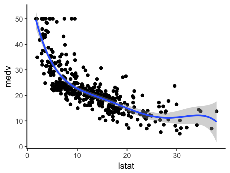
Log transformation
When you have a non-linear relationship, you can also try a logarithm transformation of the predictor variables:
# Build the model
model <- lm(medv ~ log(lstat), data = train.data)
# Make predictions
predictions <- model %>% predict(test.data)
# Model performance
data.frame(
  RMSE = RMSE(predictions, test.data$medv),
  R2 = R2(predictions, test.data$medv)
)
## RMSE R2
## 1 5.24 0.657Visualize the data:
ggplot(train.data, aes(lstat, medv) ) +
  geom_point() +
stat_smooth(method = lm, formula = y ~ log(x))![]()
Spline regression
Polynomial regression only captures a certain amount of curvature in a nonlinear relationship. An alternative, and often superior, approach to modeling nonlinear relationships is to use splines (P. Bruce and Bruce 2017).
Splines provide a way to smoothly interpolate between fixed points, called knots. Polynomial regression is computed between knots. In other words, splines are series of polynomial segments strung together, joining at knots (P. Bruce and Bruce 2017).
The R package splines includes the function bs for creating a b-spline term in a regression model.
You need to specify two parameters: the degree of the polynomial and the location of the knots. In our example, we’ll place the knots at the lower quartile, the median quartile, and the upper quartile:
knots <- quantile(train.data$lstat, p = c(0.25, 0.5, 0.75))We’ll create a model using a cubic spline (degree = 3):
library(splines)
# Build the model
knots <- quantile(train.data$lstat, p = c(0.25, 0.5, 0.75))
model <- lm (medv ~ bs(lstat, knots = knots), data = train.data)
# Make predictions
predictions <- model %>% predict(test.data)
# Model performance
data.frame(
  RMSE = RMSE(predictions, test.data$medv),
  R2 = R2(predictions, test.data$medv)
)
## RMSE R2
## 1 4.97 0.688Note that, the coefficients for a spline term are not interpretable.
Visualize the cubic spline as follow:
ggplot(train.data, aes(lstat, medv) ) +
  geom_point() +
  stat_smooth(method = lm, formula = y ~ splines::bs(x, df = 3))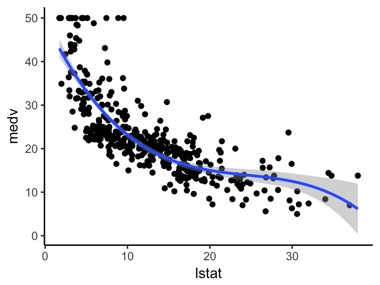
Generalized additive models
Once you have detected a non-linear relationship in your data, the polynomial terms may not be flexible enough to capture the relationship, and spline terms require specifying the knots.
Generalized additive models, or GAM, are a technique to automatically fit a spline regression. This can be done using the mgcv R package:
library(mgcv)
# Build the model
model <- gam(medv ~ s(lstat), data = train.data)
# Make predictions
predictions <- model %>% predict(test.data)
# Model performance
data.frame(
  RMSE = RMSE(predictions, test.data$medv),
  R2 = R2(predictions, test.data$medv)
)
## RMSE R2
## 1 5.02 0.684The term s(lstat) tells the gam() function to find the “best” knots for a spline term.
Visualize the data:
ggplot(train.data, aes(lstat, medv) ) +
  geom_point() +
  stat_smooth(method = gam, formula = y ~ s(x))
Comparing the models
From analyzing the RMSE and the R2 metrics of the different models, it can be seen that the polynomial regression, the spline regression and the generalized additive models outperform the linear regression model and the log transformation approaches.
Discussion
This chapter describes how to compute non-linear regression models using R.
References
Bruce, Peter, and Andrew Bruce. 2017. Practical Statistics for Data Scientists. O’Reilly Media.