


SVM Model: Support Vector Machine Essentials
Support Vector Machine (or SVM) is a machine learning technique used for classification tasks. Briefly, SVM works by identifying the optimal decision boundary that separates data points from different groups (or classes), and then predicts the class of new observations based on this separation boundary.
Depending on the situations, the different groups might be separable by a linear straight line or by a non-linear boundary line.
Support vector machine methods can handle both linear and non-linear class boundaries. It can be used for both two-class and multi-class classification problems.
In real life data, the separation boundary is generally nonlinear. Technically, the SVM algorithm perform a non-linear classification using what is called the kernel trick. The most commonly used kernel transformations are polynomial kernel and radial kernel.
Note that, there is also an extension of the SVM for regression, called support vector regression.
In this chapter, we’ll describe how to build SVM classifier using the caret R package.
Contents:

Loading required R packages
tidyversefor easy data manipulation and visualizationcaretfor easy machine learning workflow
library(tidyverse)
library(caret)
Example of data set
Data set: PimaIndiansDiabetes2 [in mlbench package], introduced in Chapter @ref(classification-in-r), for predicting the probability of being diabetes positive based on multiple clinical variables.
We’ll randomly split the data into training set (80% for building a predictive model) and test set (20% for evaluating the model). Make sure to set seed for reproducibility.
# Load the data
data("PimaIndiansDiabetes2", package = "mlbench")
pima.data <- na.omit(PimaIndiansDiabetes2)
# Inspect the data
sample_n(pima.data, 3)
# Split the data into training and test set
set.seed(123)
training.samples <- pima.data$diabetes %>%
  createDataPartition(p = 0.8, list = FALSE)
train.data  <- pima.data[training.samples, ]
test.data <- pima.data[-training.samples, ]
SVM linear classifier
In the following example variables are normalized to make their scale comparable. This is automatically done before building the SVM classifier by setting the option preProcess = c("center","scale").
# Fit the model on the training set
set.seed(123)
model <- train(
  diabetes ~., data = train.data, method = "svmLinear",
  trControl = trainControl("cv", number = 10),
  preProcess = c("center","scale")
  )
# Make predictions on the test data
predicted.classes <- model %>% predict(test.data)
head(predicted.classes)
## [1] neg pos neg pos pos neg
## Levels: neg pos# Compute model accuracy rate
mean(predicted.classes == test.data$diabetes)## [1] 0.782Note that, there is a tuning parameter C, also known as Cost, that determines the possible misclassifications. It essentially imposes a penalty to the model for making an error: the higher the value of C, the less likely it is that the SVM algorithm will misclassify a point.
By default caret builds the SVM linear classifier using C = 1. You can check this by typing model in R console.
It’s possible to automatically compute SVM for different values of `C and to choose the optimal one that maximize the model cross-validation accuracy.
The following R code compute SVM for a grid values of C and choose automatically the final model for predictions:
# Fit the model on the training set
set.seed(123)
model <- train(
diabetes ~., data = train.data, method = "svmLinear",
trControl = trainControl("cv", number = 10),
tuneGrid = expand.grid(C = seq(0, 2, length = 20)),
preProcess = c("center","scale")
)
# Plot model accuracy vs different values of Cost
plot(model)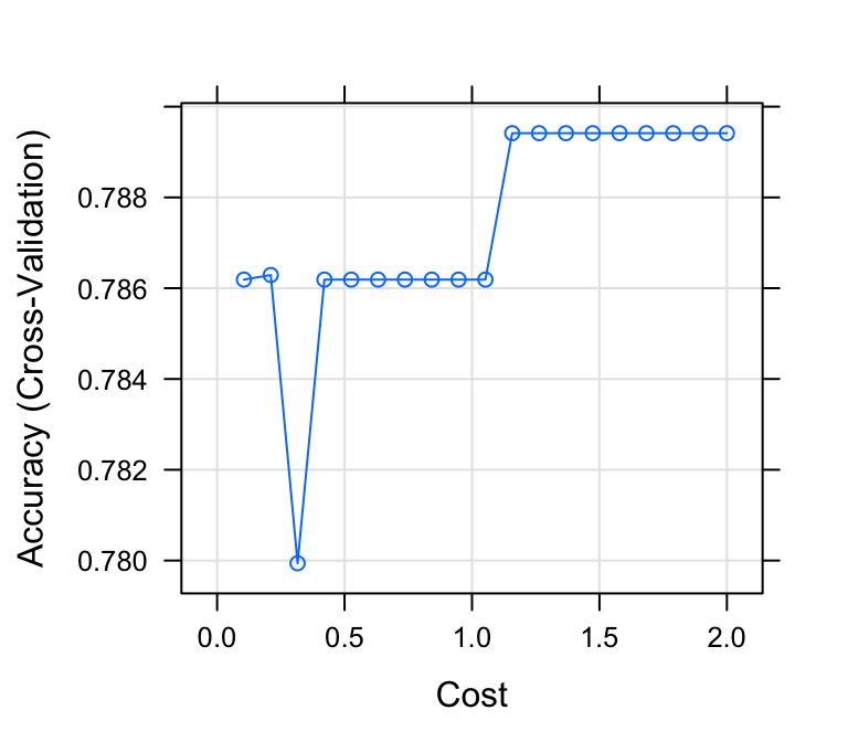
# Print the best tuning parameter C that
# maximizes model accuracy
model$bestTune## C
## 12 1.16# Make predictions on the test data
predicted.classes <- model %>% predict(test.data)
# Compute model accuracy rate
mean(predicted.classes == test.data$diabetes)
## [1] 0.782SVM classifier using Non-Linear Kernel
To build a non-linear SVM classifier, we can use either polynomial kernel or radial kernel function. Again, the caret package can be used to easily computes the polynomial and the radial SVM non-linear models.
The package automatically choose the optimal values for the model tuning parameters, where optimal is defined as values that maximize the model accuracy.
- Computing SVM using radial basis kernel:
# Fit the model on the training set
set.seed(123)
model <- train(
  diabetes ~., data = train.data, method = "svmRadial",
  trControl = trainControl("cv", number = 10),
  preProcess = c("center","scale"),
  tuneLength = 10
  )
# Print the best tuning parameter sigma and C that
# maximizes model accuracy
model$bestTune
## sigma C
## 1 0.136 0.25# Make predictions on the test data
predicted.classes <- model %>% predict(test.data)
# Compute model accuracy rate
mean(predicted.classes == test.data$diabetes)## [1] 0.795- Computing SVM using polynomial basis kernel:
# Fit the model on the training set
set.seed(123)
model <- train(
  diabetes ~., data = train.data, method = "svmPoly",
  trControl = trainControl("cv", number = 10),
  preProcess = c("center","scale"),
  tuneLength = 4
  )
# Print the best tuning parameter sigma and C that
# maximizes model accuracy
model$bestTune
## degree scale C
## 8 1 0.01 2# Make predictions on the test data
predicted.classes <- model %>% predict(test.data)
# Compute model accuracy rate
mean(predicted.classes == test.data$diabetes)## [1] 0.795In our examples, it can be seen that the SVM classifier using non-linear kernel gives a better result compared to the linear model.
Discussion
This chapter describes how to use support vector machine for classification tasks. Other alternatives exist, such as logistic regression (Chapter @ref(logistic-regression)).
You need to assess the performance of different methods on your data in order to choose the best one.