CART Model: Decision Tree Essentials
The decision tree method is a powerful and popular predictive machine learning technique that is used for both classification and regression. So, it is also known as Classification and Regression Trees (CART).
Note that the R implementation of the CART algorithm is called RPART (Recursive Partitioning And Regression Trees) available in a package of the same name.
In this chapter we’ll describe the basics of tree models and provide R codes to compute classification and regression trees.
Contents:
Loading required R packages
tidyversefor easy data manipulation and visualizationcaretfor easy machine learning workflowrpartfor computing decision tree models
library(tidyverse)
library(caret)
library(rpart)
Decision tree algorithm
Basics and visual representation
The algorithm of decision tree models works by repeatedly partitioning the data into multiple sub-spaces, so that the outcomes in each final sub-space is as homogeneous as possible. This approach is technically called recursive partitioning.
The produced result consists of a set of rules used for predicting the outcome variable, which can be either:
- a continuous variable, for regression trees
- a categorical variable, for classification trees
The decision rules generated by the CART predictive model are generally visualized as a binary tree.
The following example represents a tree model predicting the species of iris flower based on the length (in cm) and width of sepal and petal.
library(rpart)
model <- rpart(Species ~., data = iris)
par(xpd = NA) # otherwise on some devices the text is clipped
plot(model)
text(model, digits = 3)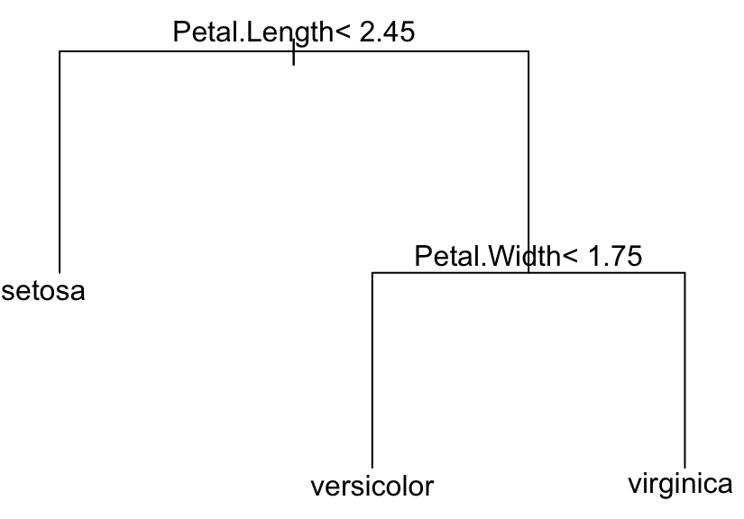
The plot shows the different possible splitting rules that can be used to effectively predict the type of outcome (here, iris species). For example, the top split assigns observations having Petal.length < 2.45 to the left branch, where the predicted species are setosa.
The different rules in tree can be printed as follow:
print(model, digits = 2)## n= 150
##
## node), split, n, loss, yval, (yprob)
## * denotes terminal node
##
## 1) root 150 100 setosa (0.333 0.333 0.333)
## 2) Petal.Length< 2.5 50 0 setosa (1.000 0.000 0.000) *
## 3) Petal.Length>=2.5 100 50 versicolor (0.000 0.500 0.500)
## 6) Petal.Width< 1.8 54 5 versicolor (0.000 0.907 0.093) *
## 7) Petal.Width>=1.8 46 1 virginica (0.000 0.022 0.978) *These rules are produced by repeatedly splitting the predictor variables, starting with the variable that has the highest association with the response variable. The process continues until some predetermined stopping criteria are met.
The resulting tree is composed of decision nodes, branches and leaf nodes. The tree is placed from upside to down, so the root is at the top and leaves indicating the outcome is put at the bottom.
Each decision node corresponds to a single input predictor variable and a split cutoff on that variable. The leaf nodes of the tree are the outcome variable which is used to make predictions.
The tree grows from the top (root), at each node the algorithm decides the best split cutoff that results to the greatest purity (or homogeneity) in each subpartition.
The tree will stop growing by the following three criteria (Zhang 2016):
- all leaf nodes are pure with a single class;
- a pre-specified minimum number of training observations that cannot be assigned to each leaf nodes with any splitting methods;
- The number of observations in the leaf node reaches the pre-specified minimum one.
A fully grown tree will overfit the training data and the resulting model might not be performant for predicting the outcome of new test data. Techniques, such as pruning, are used to control this problem.
Choosing the trees split points
Technically, for regression modeling, the split cutoff is defined so that the residual sum of squared error (RSS) is minimized across the training samples that fall within the subpartition.
Recall that, the RSS is the sum of the squared difference between the observed outcome values and the predicted ones, RSS = sum((Observeds - Predicteds)^2). See Chapter @ref(linear-regression)
In classification settings, the split point is defined so that the population in subpartitions are pure as much as possible. Two measures of purity are generally used, including the Gini index and the entropy (or information gain).
For a given subpartition, Gini = sum(p(1-p)) and entropy = -1*sum(p*log(p)), where p is the proportion of misclassified observations within the subpartition.
The sum is computed across the different categories or classes in the outcome variable. The Gini index and the entropy varie from 0 (greatest purity) to 1 (maximum degree of impurity)
Making predictions
The different rule sets established in the tree are used to predict the outcome of a new test data.
The following R code predict the species of a new collected iris flower:
newdata <- data.frame(
  Sepal.Length = 6.5, Sepal.Width = 3.0,
  Petal.Length = 5.2, Petal.Width = 2.0
)
model %>% predict(newdata, "class")
## 1
## virginica
## Levels: setosa versicolor virginicaThe new data is predicted to be virginica.
Classification trees
Example of data set
Data set: PimaIndiansDiabetes2 [in mlbench package], introduced in Chapter @ref(classification-in-r), for predicting the probability of being diabetes positive based on multiple clinical variables.
We’ll randomly split the data into training set (80% for building a predictive model) and test set (20% for evaluating the model). Make sure to set seed for reproducibility.
# Load the data and remove NAs
data("PimaIndiansDiabetes2", package = "mlbench")
PimaIndiansDiabetes2 <- na.omit(PimaIndiansDiabetes2)
# Inspect the data
sample_n(PimaIndiansDiabetes2, 3)
# Split the data into training and test set
set.seed(123)
training.samples <- PimaIndiansDiabetes2$diabetes %>%
  createDataPartition(p = 0.8, list = FALSE)
train.data  <- PimaIndiansDiabetes2[training.samples, ]
test.data <- PimaIndiansDiabetes2[-training.samples, ]
Fully grown trees
Here, we’ll create a fully grown tree showing all predictor variables in the data set.
# Build the model
set.seed(123)
model1 <- rpart(diabetes ~., data = train.data, method = "class")
# Plot the trees
par(xpd = NA) # Avoid clipping the text in some device
plot(model1)
text(model1, digits = 3)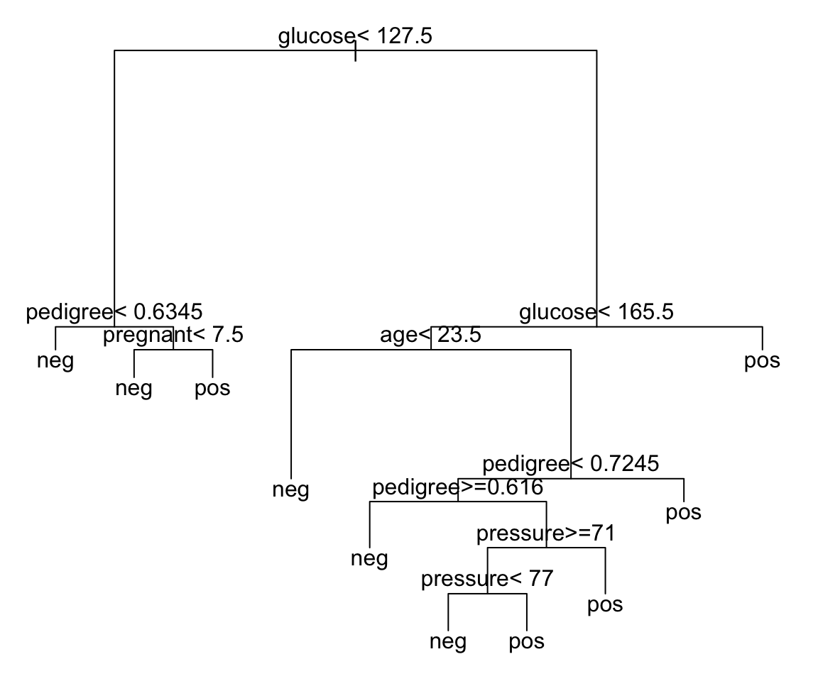
# Make predictions on the test data
predicted.classes <- model1 %>%
  predict(test.data, type = "class")
head(predicted.classes)
## 21 25 28 29 32 36
## neg pos neg pos pos neg
## Levels: neg pos# Compute model accuracy rate on test data
mean(predicted.classes == test.data$diabetes)## [1] 0.782The overall accuracy of our tree model is 78%, which is not so bad.
However, this full tree including all predictor appears to be very complex and can be difficult to interpret in the situation where you have a large data sets with multiple predictors.
Additionally, it is easy to see that, a fully grown tree will overfit the training data and might lead to poor test set performance.
A strategy to limit this overfitting is to prune back the tree resulting to a simpler tree with fewer splits and better interpretation at the cost of a little bias (James et al. 2014, P. Bruce and Bruce (2017)).
Pruning the tree
Briefly, our goal here is to see if a smaller subtree can give us comparable results to the fully grown tree. If yes, we should go for the simpler tree because it reduces the likelihood of overfitting.
One possible robust strategy of pruning the tree (or stopping the tree to grow) consists of avoiding splitting a partition if the split does not significantly improves the overall quality of the model.
In rpart package, this is controlled by the complexity parameter (cp), which imposes a penalty to the tree for having two many splits. The default value is 0.01. The higher the cp, the smaller the tree.
A too small value of cp leads to overfitting and a too large cp value will result to a too small tree. Both cases decrease the predictive performance of the model.
An optimal cp value can be estimated by testing different cp values and using cross-validation approaches to determine the corresponding prediction accuracy of the model. The best cp is then defined as the one that maximize the cross-validation accuracy (Chapter @ref(cross-validation)).
Pruning can be easily performed in the caret package workflow, which invokes the rpart method for automatically testing different possible values of cp, then choose the optimal cp that maximize the cross-validation (“cv”) accuracy, and fit the final best CART model that explains the best our data.
You can use the following arguments in the function train() [from caret package]:
trControl, to set up 10-fold cross validationtuneLength, to specify the number of possiblecpvalues to evaluate. Default value is 3, here we’ll use 10.
# Fit the model on the training set
set.seed(123)
model2 <- train(
diabetes ~., data = train.data, method = "rpart",
trControl = trainControl("cv", number = 10),
tuneLength = 10
)
# Plot model accuracy vs different values of
# cp (complexity parameter)
plot(model2)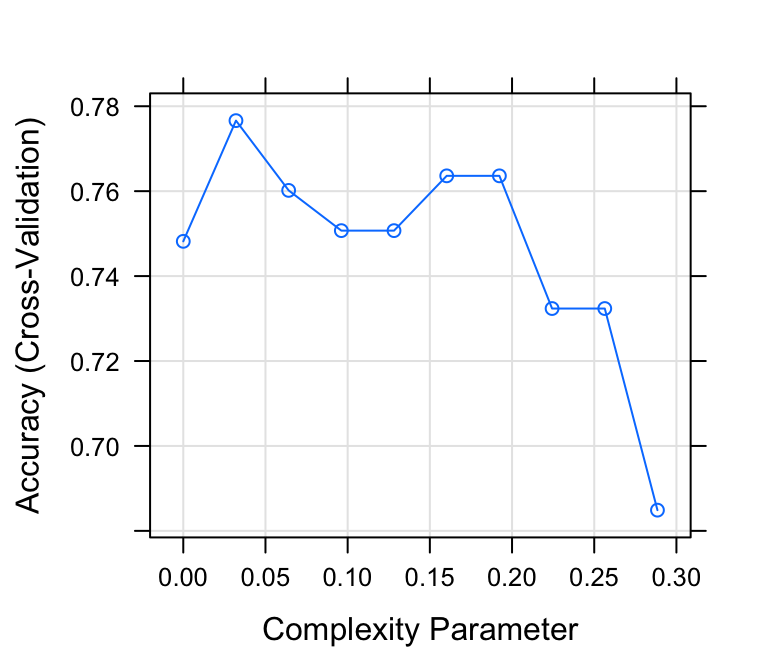
# Print the best tuning parameter cp that
# maximizes the model accuracy
model2$bestTune## cp
## 2 0.0321# Plot the final tree model
par(xpd = NA) # Avoid clipping the text in some device
plot(model2$finalModel)
text(model2$finalModel, digits = 3)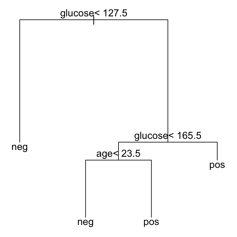
# Decision rules in the model
model2$finalModel## n= 314
##
## node), split, n, loss, yval, (yprob)
## * denotes terminal node
##
## 1) root 314 104 neg (0.6688 0.3312)
## 2) glucose< 128 188 26 neg (0.8617 0.1383) *
## 3) glucose>=128 126 48 pos (0.3810 0.6190)
## 6) glucose< 166 88 44 neg (0.5000 0.5000)
## 12) age< 23.5 16 1 neg (0.9375 0.0625) *
## 13) age>=23.5 72 29 pos (0.4028 0.5972) *
## 7) glucose>=166 38 4 pos (0.1053 0.8947) *# Make predictions on the test data
predicted.classes <- model2 %>% predict(test.data)
# Compute model accuracy rate on test data
mean(predicted.classes == test.data$diabetes)
## [1] 0.795From the output above, it can be seen that the best value for the complexity parameter (cp) is 0.032, allowing a simpler tree, easy to interpret, with an overall accuracy of 79%, which is comparable to the accuracy (78%) that we have obtained with the full tree. The prediction accuracy of the pruned tree is even better compared to the full tree.
Taken together, we should go for this simpler model.
Regression trees
Previously, we described how to build a classification tree for predicting the group (i.e. class) of observations. In this section, we’ll describe how to build a tree for predicting a continuous variable, a method called regression analysis (Chapter @ref(regression-analysis)).
The R code is identical to what we have seen in previous sections. Pruning should be also applied here to limit overfiting.
Similarly to classification trees, the following R code uses the caret package to build regression trees and to predict the output of a new test data set.
Example of data set
Data set: We’ll use the Boston data set [in MASS package], introduced in Chapter @ref(regression-analysis), for predicting the median house value (mdev), in Boston Suburbs, using different predictor variables.
We’ll randomly split the data into training set (80% for building a predictive model) and test set (20% for evaluating the model). Make sure to set seed for reproducibility.
# Load the data
data("Boston", package = "MASS")
# Inspect the data
sample_n(Boston, 3)
# Split the data into training and test set
set.seed(123)
training.samples <- Boston$medv %>%
  createDataPartition(p = 0.8, list = FALSE)
train.data  <- Boston[training.samples, ]
test.data <- Boston[-training.samples, ]
Create the regression tree
Here, the best cp value is the one that minimize the prediction error RMSE (root mean squared error).
The prediction error is measured by the RMSE, which corresponds to the average difference between the observed known values of the outcome and the predicted value by the model. RMSE is computed as RMSE = mean((observeds - predicteds)^2) %>% sqrt(). The lower the RMSE, the better the model.
Choose the best cp value:
# Fit the model on the training set
set.seed(123)
model <- train(
  medv ~., data = train.data, method = "rpart",
  trControl = trainControl("cv", number = 10),
  tuneLength = 10
  )
# Plot model error vs different values of
# cp (complexity parameter)
plot(model)
# Print the best tuning parameter cp that
# minimize the model RMSE
model$bestTune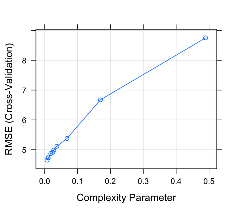
Plot the final tree model:
# Plot the final tree model
par(xpd = NA) # Avoid clipping the text in some device
plot(model$finalModel)
text(model$finalModel, digits = 3)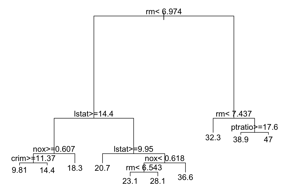
# Decision rules in the model
model$finalModel
# Make predictions on the test data
predictions <- model %>% predict(test.data)
head(predictions)
# Compute the prediction error RMSE
RMSE(predictions, test.data$medv)
Conditionnal inference tree
The conditional inference tree (ctree) uses significance test methods to select and split recursively the most related predictor variables to the outcome. This can limit overfitting compared to the classical rpart algorithm.
At each splitting step, the algorithm stops if there is no dependence between predictor variables and the outcome variable. Otherwise the variable that is the most associated to the outcome is selected for splitting.
The conditional tree can be easily computed using the caret workflow, which will invoke the function ctree() available in the party package.
- Demo data:
PimaIndiansDiabetes2. First split the data into training (80%) and test set (20%)
# Load the data
data("PimaIndiansDiabetes2", package = "mlbench")
pima.data <- na.omit(PimaIndiansDiabetes2)
# Split the data into training and test set
set.seed(123)
training.samples <- pima.data$diabetes %>%
  createDataPartition(p = 0.8, list = FALSE)
train.data  <- pima.data[training.samples, ]
test.data <- pima.data[-training.samples, ]- Build conditional trees using the tuning parameters
maxdepthandmincriterionfor controlling the tree size.caretpackage selects automatically the optimal tuning values for your data, but here we’ll specifymaxdepthandmincriterion.
The following example create a classification tree:
library(party)
set.seed(123)
model <- train(
  diabetes ~., data = train.data, method = "ctree2",
  trControl = trainControl("cv", number = 10),
  tuneGrid = expand.grid(maxdepth = 3, mincriterion = 0.95 )
  )
plot(model$finalModel)
# Make predictions on the test data
predicted.classes <- model %>% predict(test.data)
# Compute model accuracy rate on test data
mean(predicted.classes == test.data$diabetes)
## [1] 0.744The p-value indicates the association between a given predictor variable and the outcome variable. For example, the first decision node at the top shows that glucose is the variable that is most strongly associated with diabetes with a p value < 0.001, and thus is selected as the first node.
Discussion
This chapter describes how to build classification and regression tree in R. Trees provide a visual tool that are very easy to interpret and to explain to people.
Tree models might be very performant compared to the linear regression model (Chapter @ref(linear-regression)), when there is a highly non-linear and complex relationships between the outcome variable and the predictors.
However, building only one single tree from a training data set might results to a less performant predictive model. A single tree is unstable and the structure might be altered by small changes in the training data.
For example, the exact split point of a given predictor variable and the predictor to be selected at each step of the algorithm are strongly dependent on the training data set. Using a slightly different training data may alter the first variable to split in, and the structure of the tree can be completely modified.
Other machine learning algorithms - including bagging, random forest and boosting - can be used to build multiple different trees from one single data set leading to a better predictive performance. But, with these methods the interpretability observed for a single tree is lost. Note that all these above mentioned strategies are based on the CART algorithm. See Chapter @ref(bagging-and-random-forest) and @ref(boosting).
References
Bruce, Peter, and Andrew Bruce. 2017. Practical Statistics for Data Scientists. O’Reilly Media.
James, Gareth, Daniela Witten, Trevor Hastie, and Robert Tibshirani. 2014. An Introduction to Statistical Learning: With Applications in R. Springer Publishing Company, Incorporated.
Zhang, Zhongheng. 2016. “Decision Tree Modeling Using R.” Annals of Translational Medicine 4 (15).


