


Bagging and Random Forest Essentials
In the Chapter @ref(decision-tree-models), we have described how to build decision trees for predictive modeling.
The standard decision tree model, CART for classification and regression trees, build only one single tree, which is then used to predict the outcome of new observations. The output of this strategy is very unstable and the tree structure might be severally affected by a small change in the training data set.
There are different powerful alternatives to the classical CART algorithm, including bagging, Random Forest and boosting.
Bagging stands for bootstrap aggregating. It consists of building multiple different decision tree models from a single training data set by repeatedly using multiple bootstrapped subsets of the data and averaging the models. Here, each tree is build independently to the others. Read more on bootstrapping in the Chapter @ref(bootstrap-resampling).
Random Forest algorithm, is one of the most commonly used and the most powerful machine learning techniques. It is a special type of bagging applied to decision trees.
Compared to the standard CART model (Chapter @ref(decision-tree-models)), the random forest provides a strong improvement, which consists of applying bagging to the data and bootstrap sampling to the predictor variables at each split (James et al. 2014, P. Bruce and Bruce (2017)). This means that at each splitting step of the tree algorithm, a random sample of n predictors is chosen as split candidates from the full set of the predictors.
Random forest can be used for both classification (predicting a categorical variable) and regression (predicting a continuous variable).
In this chapter, we’ll describe how to compute random forest algorithm in R for building a powerful predictive model. Additionally, you’ll learn how to rank the predictor variable according to their importance in contributing to the model accuracy.
Contents:

Loading required R packages
tidyversefor easy data manipulation and visualizationcaretfor easy machine learning workflowrandomForestfor computing random forest algorithm
library(tidyverse)
library(caret)
library(randomForest)
Classification
Example of data set
Data set: PimaIndiansDiabetes2 [in mlbench package], introduced in Chapter @ref(classification-in-r), for predicting the probability of being diabetes positive based on multiple clinical variables.
Randomly split the data into training set (80% for building a predictive model) and test set (20% for evaluating the model). Make sure to set seed for reproducibility.
# Load the data and remove NAs
data("PimaIndiansDiabetes2", package = "mlbench")
PimaIndiansDiabetes2 <- na.omit(PimaIndiansDiabetes2)
# Inspect the data
sample_n(PimaIndiansDiabetes2, 3)
# Split the data into training and test set
set.seed(123)
training.samples <- PimaIndiansDiabetes2$diabetes %>%
  createDataPartition(p = 0.8, list = FALSE)
train.data  <- PimaIndiansDiabetes2[training.samples, ]
test.data <- PimaIndiansDiabetes2[-training.samples, ]
Computing random forest classifier
We’ll use the caret workflow, which invokes the randomforest() function [randomForest package], to automatically select the optimal number (mtry) of predictor variables randomly sampled as candidates at each split, and fit the final best random forest model that explains the best our data.
We’ll use the following arguments in the function train():
trControl, to set up 10-fold cross validation
# Fit the model on the training set
set.seed(123)
model <- train(
  diabetes ~., data = train.data, method = "rf",
  trControl = trainControl("cv", number = 10),
  importance = TRUE
  )
# Best tuning parameter
model$bestTune
## mtry
## 3 8# Final model
model$finalModel##
## Call:
## randomForest(x = x, y = y, mtry = param$mtry, importance = TRUE)
## Type of random forest: classification
## Number of trees: 500
## No. of variables tried at each split: 8
##
## OOB estimate of error rate: 22%
## Confusion matrix:
## neg pos class.error
## neg 185 25 0.119
## pos 44 60 0.423# Make predictions on the test data
predicted.classes <- model %>% predict(test.data)
head(predicted.classes)## [1] neg pos neg neg pos neg
## Levels: neg pos# Compute model accuracy rate
mean(predicted.classes == test.data$diabetes)## [1] 0.808By default, 500 trees are trained. The optimal number of variables sampled at each split is 8.
Each bagged tree makes use of around two-thirds of the observations. The remaining one-third of the observations not used to fit a given bagged tree are referred to as the out-of-bag (OOB) observations (James et al. 2014).
For a given tree, the out-of-bag (OOB) error is the model error in predicting the data left out of the training set for that tree (P. Bruce and Bruce 2017). OOB is a very straightforward way to estimate the test error of a bagged model, without the need to perform cross-validation or the validation set approach.
In our example, the OBB estimate of error rate is 24%.
The prediction accuracy on new test data is 79%, which is good.
Variable importance
The importance of each variable can be printed using the function importance() [randomForest package]:
importance(model$finalModel)## neg pos MeanDecreaseAccuracy MeanDecreaseGini
## pregnant 11.57 0.318 10.36 8.86
## glucose 38.93 28.437 46.17 53.30
## pressure -1.94 0.846 -1.06 8.09
## triceps 6.19 3.249 6.85 9.92
## insulin 8.65 -2.037 6.01 12.43
## mass 7.71 2.299 7.57 14.58
## pedigree 6.57 1.083 5.66 14.50
## age 9.51 12.310 15.75 16.76The result shows:
MeanDecreaseAccuracy, which is the average decrease of model accuracy in predicting the outcome of the out-of-bag samples when a specific variable is excluded from the model.MeanDecreaseGini, which is the average decrease in node impurity that results from splits over that variable. The Gini impurity index is only used for classification problem. In the regression the node impurity is measured by training set RSS. These measures, calculated using the training set, are less reliable than a measure calculated on out-of-bag data. See Chapter @ref(decision-tree-models) for node impurity measures (Gini index and RSS).
Note that, by default (argument importance = FALSE), randomForest only calculates the Gini impurity index. However, computing the model accuracy by variable (argument importance = TRUE) requires supplementary computations which might be time consuming in the situations, where thousands of models (trees) are being fitted.
Variables importance measures can be plotted using the function varImpPlot() [randomForest package]:
# Plot MeanDecreaseAccuracy
varImpPlot(model$finalModel, type = 1)
# Plot MeanDecreaseGini
varImpPlot(model$finalModel, type = 2)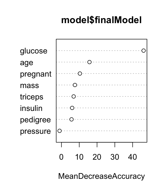
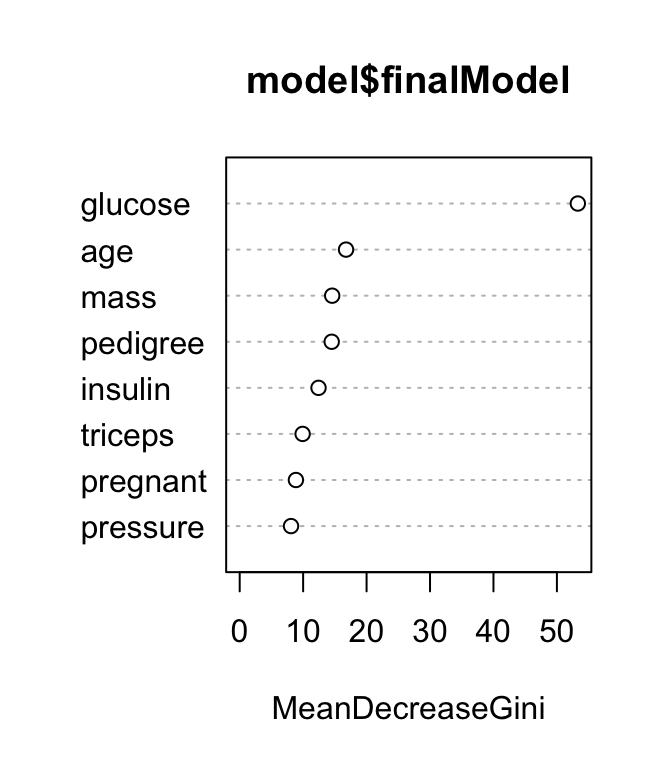
The results show that across all of the trees considered in the random forest, the glucose and age variables are the two most important variables.
The function varImp() [in caret] displays the importance of variables in percentage:
varImp(model)## rf variable importance
##
## Importance
## glucose 100.0
## age 33.5
## pregnant 19.0
## mass 16.2
## triceps 15.4
## pedigree 12.8
## insulin 11.2
## pressure 0.0Regression
Similarly, you can build a random forest model to perform regression, that is to predict a continuous variable.
Example of data set
We’ll use the Boston data set [in MASS package], introduced in Chapter @ref(regression-analysis), for predicting the median house value (mdev), in Boston Suburbs, using different predictor variables.
Randomly split the data into training set (80% for building a predictive model) and test set (20% for evaluating the model).
# Load the data
data("Boston", package = "MASS")
# Inspect the data
sample_n(Boston, 3)
# Split the data into training and test set
set.seed(123)
training.samples <- Boston$medv %>%
  createDataPartition(p = 0.8, list = FALSE)
train.data  <- Boston[training.samples, ]
test.data <- Boston[-training.samples, ]
Computing random forest regression trees
Here the prediction error is measured by the RMSE, which corresponds to the average difference between the observed known values of the outcome and the predicted value by the model. RMSE is computed as RMSE = mean((observeds - predicteds)^2) %>% sqrt(). The lower the RMSE, the better the model.
# Fit the model on the training set
set.seed(123)
model <- train(
  medv ~., data = train.data, method = "rf",
  trControl = trainControl("cv", number = 10)
  )
# Best tuning parameter mtry
model$bestTune
# Make predictions on the test data
predictions <- model %>% predict(test.data)
head(predictions)
# Compute the average prediction error RMSE
RMSE(predictions, test.data$medv)
Hyperparameters
Note that, the random forest algorithm has a set of hyperparameters that should be tuned using cross-validation to avoid overfitting.
These include:
nodesize: Minimum size of terminal nodes. Default value for classification is 1 and default for regression is 5.maxnodes: Maximum number of terminal nodes trees in the forest can have. If not given, trees are grown to the maximum possible (subject to limits by nodesize).
Ignoring these parameters might lead to overfitting on noisy data set (P. Bruce and Bruce 2017). Cross-validation can be used to test different values, in order to select the optimal value.
Hyperparameters can be tuned manually using the caret package. For a given parameter, the approach consists of fitting many models with different values of the parameters and then comparing the models.
The following example tests different values of nodesize using the PimaIndiansDiabetes2 data set for classification:
(This will take 1-2 minutes execution time)
data("PimaIndiansDiabetes2", package = "mlbench")
models <- list()
for (nodesize in c(1, 2, 4, 8)) {
    set.seed(123)
    model <- train(
      diabetes~., data = na.omit(PimaIndiansDiabetes2), method="rf",
      trControl = trainControl(method="cv", number=10),
      metric = "Accuracy",
      nodesize = nodesize
      )
    model.name <- toString(nodesize)
    models[[model.name]] <- model
}
# Compare results
resamples(models) %>% summary(metric = "Accuracy")
##
## Call:
## summary.resamples(object = ., metric = "Accuracy")
##
## Models: 1, 2, 4, 8
## Number of resamples: 10
##
## Accuracy
## Min. 1st Qu. Median Mean 3rd Qu. Max. NA's
## 1 0.692 0.750 0.785 0.793 0.840 0.897 0
## 2 0.692 0.744 0.808 0.788 0.841 0.850 0
## 4 0.692 0.744 0.795 0.786 0.825 0.846 0
## 8 0.692 0.750 0.808 0.796 0.841 0.897 0It can be seen that, using a nodesize value of 2 or 8 leads to the most median accuracy value.
Discussion
This chapter describes the basics of bagging and random forest machine learning algorithms. We also provide practical examples in R for classification and regression analyses.
Another alternative to bagging and random forest is boosting (Chapter @ref(boosting)).
References
Bruce, Peter, and Andrew Bruce. 2017. Practical Statistics for Data Scientists. O’Reilly Media.
James, Gareth, Daniela Witten, Trevor Hastie, and Robert Tibshirani. 2014. An Introduction to Statistical Learning: With Applications in R. Springer Publishing Company, Incorporated.