


Multidimensional Scaling Essentials: Algorithms and R Code
Multidimensional scaling (MDS) is a multivariate data analysis approach that is used to visualize the similarity/dissimilarity between samples by plotting points in two dimensional plots.
MDS returns an optimal solution to represent the data in a lower-dimensional space, where the number of dimensions k is pre-specified by the analyst. For example, choosing k = 2 optimizes the object locations for a two-dimensional scatter plot.
An MDS algorithm takes as an input data the dissimilarity matrix, representing the distances between pairs of objects.
The input data for MDS is a dissimilarity matrix representing the distances between pairs of objects.
This article describes MDS algorithms and provides R code to compute MDS.
Contents:
Types of MDS algorithms
There are different types of MDS algorithms, including
- Classical multidimensional scaling
Preserves the original distance metric, between points, as well as possible. That is the fitted distances on the MDS map and the original distances are in the same metric. Classic MDS belongs to the so-called metric multidimensional scaling category.
It’s also known as principal coordinates analysis. It’s suitable for quantitative data.
- Non-metric multidimensional scaling
It’s also known as ordinal MDS. Here, it’s not the metric of a distance value that is important or meaningful, but its value in relation to the distances between other pairs of objects.
Ordinal MDS constructs fitted distances that are in the same rank order as the original distance. For example, if the distance of apart objects 1 and 5 rank fifth in the original distance data, then they should also rank fifth in the MDS configuration.
It’s suitable for qualitative data.
Compute MDS in R
R functions
cmdscale()[stats package]: Compute classical (metric) multidimensional scaling.isoMDS()[MASS package]: Compute Kruskal’s non-metric multidimensional scaling (one form of non-metric MDS).sammon()[MASS package]: Compute sammon’s non-linear mapping (one form of non-metric MDS).
All these functions take a distance object as the main argument and k is the desired number of dimensions in the scaled output. By default, they return two dimension solutions, but we can change that through the parameter k which defaults to 2.
Demo data
swiss data that contains fertility and socio-economic data on 47 French speaking provinces in Switzerland.
data("swiss")
head(swiss)
## Fertility Agriculture Examination Education Catholic
## Courtelary 80.2 17.0 15 12 9.96
## Delemont 83.1 45.1 6 9 84.84
## Franches-Mnt 92.5 39.7 5 5 93.40
## Moutier 85.8 36.5 12 7 33.77
## Neuveville 76.9 43.5 17 15 5.16
## Porrentruy 76.1 35.3 9 7 90.57
## Infant.Mortality
## Courtelary 22.2
## Delemont 22.2
## Franches-Mnt 20.2
## Moutier 20.3
## Neuveville 20.6
## Porrentruy 26.6Classical MDS
# Load required packages
library(magrittr)
library(dplyr)
library(ggpubr)
# Cmpute MDS
mds <- swiss %>%
  dist() %>%
  cmdscale() %>%
  as_tibble()
colnames(mds) <- c("Dim.1", "Dim.2")
# Plot MDS
ggscatter(mds, x = "Dim.1", y = "Dim.2",
          label = rownames(swiss),
          size = 1,
          repel = TRUE)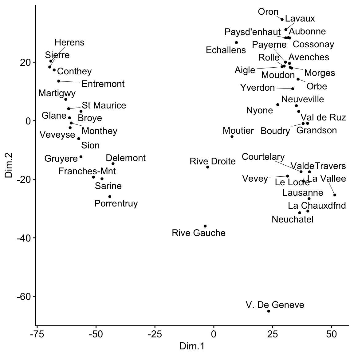
Create 3 groups using k-means clustering. Color points by groups
# K-means clustering
clust <- kmeans(mds, 3)$cluster %>%
  as.factor()
mds <- mds %>%
  mutate(groups = clust)
# Plot and color by groups
ggscatter(mds, x = "Dim.1", y = "Dim.2",
          label = rownames(swiss),
          color = "groups",
          palette = "jco",
          size = 1,
          ellipse = TRUE,
          ellipse.type = "convex",
          repel = TRUE)
Non-metric MDS
- Load general packages:
library(magrittr)
library(dplyr)
library(ggpubr)- Kruskal’s non-metric multidimensional scaling
# Cmpute MDS
library(MASS)
mds <- swiss %>%
  dist() %>%
  isoMDS() %>%
  .$points %>%
  as_tibble()
colnames(mds) <- c("Dim.1", "Dim.2")
# Plot MDS
ggscatter(mds, x = "Dim.1", y = "Dim.2",
          label = rownames(swiss),
          size = 1,
repel = TRUE)- Sammon’s non-linear mapping:
# Cmpute MDS
library(MASS)
mds <- swiss %>%
  dist() %>%
  sammon() %>%
  .$points %>%
  as_tibble()
colnames(mds) <- c("Dim.1", "Dim.2")
# Plot MDS
ggscatter(mds, x = "Dim.1", y = "Dim.2",
          label = rownames(swiss),
          size = 1,
          repel = TRUE)
Visualizing a correlation matrix using Multidimensional Scaling
MDS can be also used to reveal a hidden pattern in a correlation matrix.
Correlation actually measures similarity, but it is easy to transform it to a measure of dissimilarity. Distance between objects can be calculated as 1 - res.cor.
res.cor <- cor(mtcars, method = "spearman")
mds.cor <- (1 - res.cor) %>%
  cmdscale() %>%
  as_tibble()
colnames(mds.cor) <- c("Dim.1", "Dim.2")
ggscatter(mds.cor, x = "Dim.1", y = "Dim.2",
          size = 1,
          label = colnames(res.cor),
          repel = TRUE)
Positive correlated objects are close together on the same side of the plot.
Comparing MDS and PCA
Mathematically and conceptually, there are close correspondences between MDS and other methods used to reduce the dimensionality of complex data, such as Principal components analysis (PCA) and factor analysis.
PCA is more focused on the dimensions themselves, and seek to maximize explained variance, whereas MDS is more focused on relations among the scaled objects.
MDS projects n-dimensional data points to a (commonly) 2-dimensional space such that similar objects in the n-dimensional space will be close together on the two dimensional plot, while PCA projects a multidimensional space to the directions of maximum variability using covariance/correlation matrix to analyze the correlation between data points and variables.