Clustering Validation Statistics: 4 Vital Things Everyone Should Know - Unsupervised Machine Learning
Clustering is an unsupervised machine learning method for partitioning dataset into a set of groups or clusters. A big issue is that clustering methods will return clusters even if the data does not contain any clusters. Therefore, it’s necessary i) to assess clustering tendency before the analysis and ii) to validate the quality of the result after clustering.
A variety of measures has been proposed in the literature for evaluating clustering results. The term clustering validation is used to design the procedure of evaluating the results of a clustering algorithm.
Generally, clustering validation statistics can be categorized into 4 classes (Theodoridis and Koutroubas, 2008; G. Brock et al., 2008, Charrad et al., 2014):
Relative clustering validation, which evaluates the clustering structure by varying different parameter values for the same algorithm (e.g.,: varying the number of clusters k). It’s generally used for determining the optimal number of clusters.
External clustering validation, which consists in comparing the results of a cluster analysis to an externally known result, such as externally provided class labels. Since we know the “true” cluster number in advance, this approach is mainly used for selecting the right clustering algorithm for a specific dataset.
Internal clustering validation, which use the internal information of the clustering process to evaluate the goodness of a clustering structure without reference to external information. It can be also used for estimating the number of clusters and the appropriate clustering algorithm without any external data.
- Clustering stability validation, which is a special version of internal validation. It evaluates the consistency of a clustering result by comparing it with the clusters obtained after each column is removed, one at a time. Clustering stability measures will be described in a future chapter.
The aim of this article is to:
- describe the different methods for clustering validation
- compare the quality of clustering results obtained with different clustering algorithms
- provide R lab section for validating clustering results
In all the examples presented here, we’ll apply k-means, PAM and hierarchical clustering. Note that, the functions used in this article can be applied to evaluate the validity of any other clustering methods.
1 Required packages
The following packages will be used:
- cluster for computing PAM clustering and for analyzing cluster silhouettes
- factoextra for simplifying clustering workflows and for visualizing clusters using ggplot2 plotting system
- NbClust for determining the optimal number of clusters in the data
- fpc for computing clustering validation statistics
Install factoextra package as follow:
if(!require(devtools)) install.packages("devtools")
devtools::install_github("kassambara/factoextra")
The remaining packages can be installed using the code below:
pkgs <- c("cluster", "fpc", "NbClust")
install.packages(pkgs)
Load packages:
library(factoextra)
library(cluster)
library(fpc)
library(NbClust)
2 Data preparation
The data set iris is used. We start by excluding the column “Species” and scaling the data using the function scale():
# Load the data
data(iris)
head(iris)
## Sepal.Length Sepal.Width Petal.Length Petal.Width Species
## 1 5.1 3.5 1.4 0.2 setosa
## 2 4.9 3.0 1.4 0.2 setosa
## 3 4.7 3.2 1.3 0.2 setosa
## 4 4.6 3.1 1.5 0.2 setosa
## 5 5.0 3.6 1.4 0.2 setosa
## 6 5.4 3.9 1.7 0.4 setosa# Remove species column (5) and scale the data
iris.scaled <- scale(iris[, -5])Iris data set gives the measurements in centimeters of the variables sepal length and width and petal length and width, respectively, for 50 flowers from each of 3 species of iris. The species are Iris setosa, versicolor, and virginica.
3 Relative measures: Determine the optimal number of clusters
Many indices (more than 30) has been published in the literature for finding the right number of clusters in a dataset. The process has been covered in my previous article: Determining the optimal number of clusters.
In this section we’ll use the package NbClust which will compute, with a single function call, 30 indices for deciding the right number of clusters in the dataset:
# Compute the number of clusters
library(NbClust)
nb <- NbClust(iris.scaled, distance = "euclidean", min.nc = 2,
        max.nc = 10, method = "complete", index ="all")
# Visualize the result
library(factoextra)
fviz_nbclust(nb) + theme_minimal()## Among all indices:
## ===================
## * 2 proposed 0 as the best number of clusters
## * 1 proposed 1 as the best number of clusters
## * 2 proposed 2 as the best number of clusters
## * 18 proposed 3 as the best number of clusters
## * 3 proposed 10 as the best number of clusters
##
## Conclusion
## =========================
## * Accoridng to the majority rule, the best number of clusters is 3 .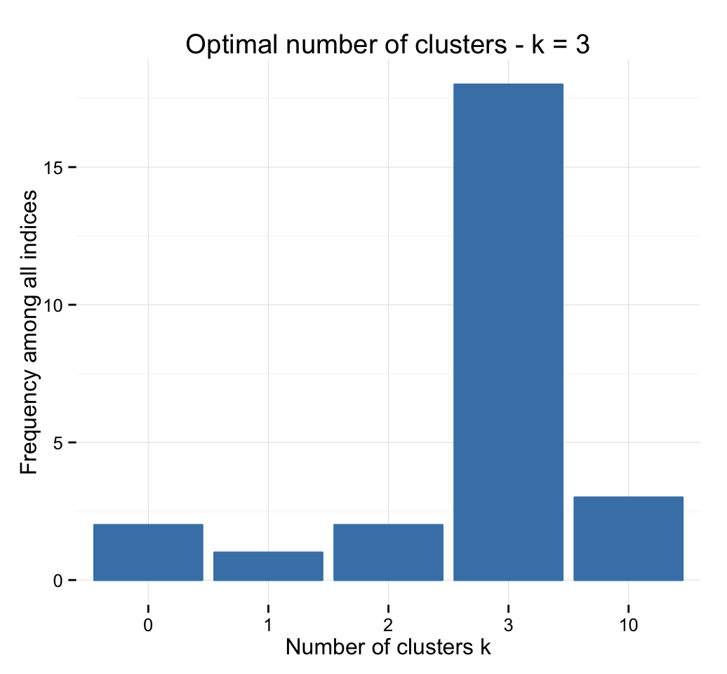
4 Clustering analysis
We’ll use the function eclust() [in factoextra] which provides several advantages as described in the previous chapter: Visual Enhancement of Clustering Analysis.
eclust() stands for enhanced clustering. It simplifies the workflow of clustering analysis and, it can be used to compute hierarchical clustering and partititioning clustering in a single line function call.
4.1 Example of partitioning method results
K-means and PAM clustering are described in this section. We’ll split the data into 3 clusters as follow:
# K-means clustering
km.res <- eclust(iris.scaled, "kmeans", k = 3,
                 nstart = 25, graph = FALSE)
# k-means group number of each observation
km.res$cluster
## [1] 1 1 1 1 1 1 1 1 1 1 1 1 1 1 1 1 1 1 1 1 1 1 1 1 1 1 1 1 1 1 1 1 1 1 1
## [36] 1 1 1 1 1 1 1 1 1 1 1 1 1 1 1 2 2 2 3 3 3 2 3 3 3 3 3 3 3 3 2 3 3 3 3
## [71] 2 3 3 3 3 2 2 2 3 3 3 3 3 3 3 2 2 3 3 3 3 3 3 3 3 3 3 3 3 3 2 3 2 2 2
## [106] 2 3 2 2 2 2 2 2 3 3 2 2 2 2 3 2 3 2 3 2 2 3 2 2 2 2 2 2 3 3 2 2 2 3 2
## [141] 2 2 3 2 2 2 3 2 2 3# Visualize k-means clusters
fviz_cluster(km.res, geom = "point", frame.type = "norm")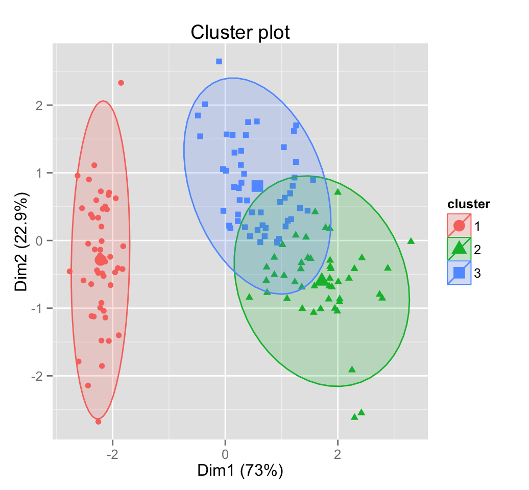
# PAM clustering
pam.res <- eclust(iris.scaled, "pam", k = 3, graph = FALSE)
pam.res$cluster
## [1] 1 1 1 1 1 1 1 1 1 1 1 1 1 1 1 1 1 1 1 1 1 1 1 1 1 1 1 1 1 1 1 1 1 1 1
## [36] 1 1 1 1 1 1 1 1 1 1 1 1 1 1 1 2 2 2 3 3 3 2 3 3 3 3 3 3 3 3 2 3 3 3 3
## [71] 3 3 3 3 3 2 2 2 3 3 3 3 3 3 3 3 2 3 3 3 3 3 3 3 3 3 3 3 3 3 2 3 2 2 2
## [106] 2 3 2 2 2 2 2 2 3 2 2 2 2 2 3 2 3 2 3 2 2 3 3 2 2 2 2 2 3 3 2 2 2 3 2
## [141] 2 2 3 2 2 2 3 2 2 3# Visualize pam clusters
fviz_cluster(pam.res, geom = "point", frame.type = "norm")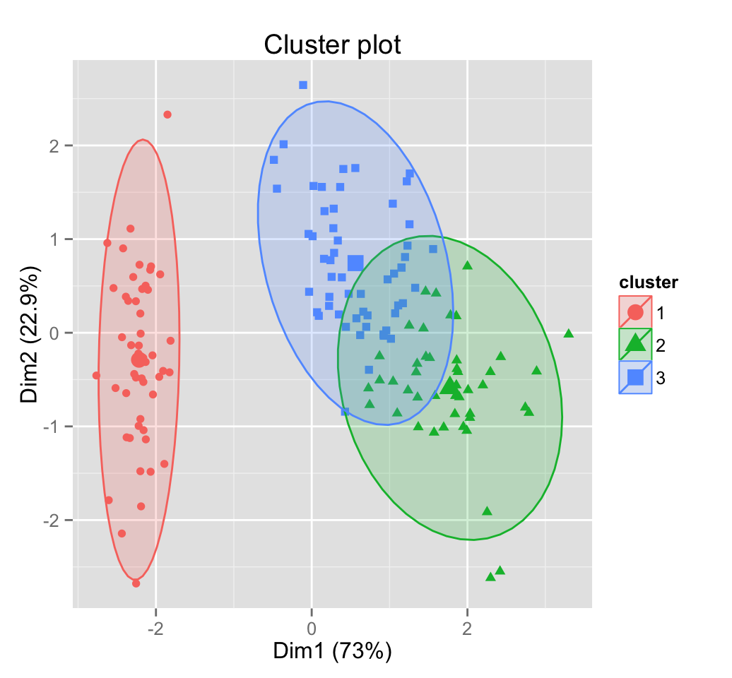
Read more about partitioning methods: Partitioning clustering
4.2 Example of hierarchical clustering results
# Enhanced hierarchical clustering
res.hc <- eclust(iris.scaled, "hclust", k = 3,
                method = "complete", graph = FALSE)
head(res.hc$cluster, 15)
## 1 2 3 4 5 6 7 8 9 10 11 12 13 14 15
## 1 1 1 1 1 1 1 1 1 1 1 1 1 1 1# Dendrogram
fviz_dend(res.hc, rect = TRUE, show_labels = FALSE) 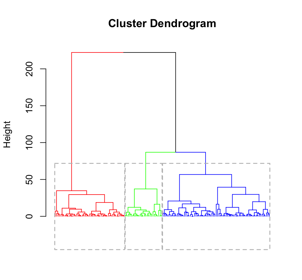
Read more about hierarchical clustering: Hierarchical clustering
5 Internal clustering validation measures
In this section, we describe the most widely used clustering validation indices. Recall that the goal of clustering algorithms is to split the dataset into clusters of objects, such that:
- the objects in the same cluster are similar as much as possible,
- and the objects in different clusters are highly distinct
That is, we want the average distance within cluster to be as small as possible; and the average distance between clusters to be as large as possible.
Internal validation measures reflect often the compactness, the connectedness and separation of the cluster partitions.
Compactness measures evaluate how close are the objects within the same cluster. A lower within-cluster variation is an indicator of a good compactness (i.e., a good clustering). The different indices for evaluating the compactness of clusters are base on distance measures such as the cluster-wise within average/median distances between observations.
- Separation measures determine how well-separated a cluster is from other clusters. The indices used as separation measures include:
- distances between cluster centers
- the pairwise minimum distances between objects in different clusters
- Connectivity corresponds to what extent items are placed in the same cluster as their nearest neighbors in the data space. The connectivity has a value between 0 and infinity and should be minimized.
Generally most of the indices used for internal clustering validation combine compactness and separation measures as follow:
\[ Index = \frac{(\alpha \times Separation)}{(\beta \times Compactness)} \]
Where \(\alpha\) and \(\beta\) are weights.
In this section, we’ll describe the two commonly used indices for assessing the goodness of clustering: silhouette width and Dunn index.
Recall that, more than 30 indices has been published in literature. They can be easily computed using the function NbClust which has been described in my previous article: Determining the optimal number of clusters.
5.1 Silhouette analysis
5.1.1 Concept and algorithm
Silhouette analysis measures how well an observation is clustered and it estimates the average distance between clusters. The silhouette plot displays a measure of how close each point in one cluster is to points in the neighboring clusters.
For each observation \(i\), the silhouette width \(s_i\) is calculated as follows:
- For each observation \(i\), calculate the average dissimilarity \(a_i\) between \(i\) and all other points of the cluster to which i belongs.
For all other clusters \(C\), to which i does not belong, calculate the average dissimilarity \(d(i, C)\) of \(i\) to all observations of C. The smallest of these \(d(i,C)\) is defined as \(b_i= \min_C d(i,C)\). The value of \(b_i\) can be seen as the dissimilarity between \(i\) and its “neighbor” cluster, i.e., the nearest one to which it does not belong.
- Finally the silhouette width of the observation \(i\) is defined by the formula: \(S_i = (b_i - a_i)/max(a_i, b_i)\).
5.1.2 Interpretation of silhouette width
Silhouette width can be interpreted as follow:
Observations with a large \(S_i\) (almost 1) are very well clustered
A small \(S_i\) (around 0) means that the observation lies between two clusters
- Observations with a negative \(S_i\) are probably placed in the wrong cluster.
5.1.3 R functions for silhouette analysis
The silhouette coefficient of observations can be computed using the function silhouette() [in cluster package]:
silhouette(x, dist, ...)- x: an integer vector containing the cluster assignment of observations
- dist: a dissimilarity object created by the function dist()
The function silhouette() returns an object, of class silhouette containing:
- The cluster number of each observation i
- The neighbor cluster of i (the cluster, not containing i, for which the average dissimilarity between its observations and i is minimal)
- The silhouette width \(s_i\) of each observation
The R code below computes silhouette analysis and draw the result using R base plot:
# Silhouette coefficient of observations
library("cluster")
sil <- silhouette(km.res$cluster, dist(iris.scaled))
head(sil[, 1:3], 10)
## cluster neighbor sil_width
## [1,] 1 3 0.7341949
## [2,] 1 3 0.5682739
## [3,] 1 3 0.6775472
## [4,] 1 3 0.6205016
## [5,] 1 3 0.7284741
## [6,] 1 3 0.6098848
## [7,] 1 3 0.6983835
## [8,] 1 3 0.7308169
## [9,] 1 3 0.4882100
## [10,] 1 3 0.6315409# Silhouette plot
plot(sil, main ="Silhouette plot - K-means")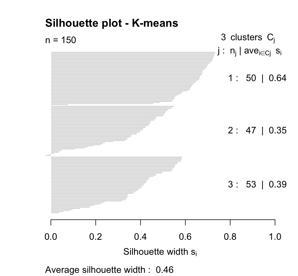
Use factoextra for elegant data visualization:
library(factoextra)
fviz_silhouette(sil)
The summary of the silhouette analysis can be computed using the function summary.silhouette() as follow:
# Summary of silhouette analysis
si.sum <- summary(sil)
# Average silhouette width of each cluster
si.sum$clus.avg.widths
## 1 2 3
## 0.6363162 0.3473922 0.3933772# The total average (mean of all individual silhouette widths)
si.sum$avg.width## [1] 0.4599482# The size of each clusters
si.sum$clus.sizes## cl
## 1 2 3
## 50 47 53Note that, if the clustering analysis is done using the function eclust(), cluster silhouettes are computed automatically and stored in the object silinfo. The results can be easily visualized as shown in the next sections.
5.1.4 Silhouette plot for k-means clustering
It’s possible to draw silhouette plot using the function fviz_silhouette() [in factoextra package], which will also print a summary of the silhouette analysis output. To avoid this, you can use the option print.summary = FALSE.
# Default plot
fviz_silhouette(km.res)## cluster size ave.sil.width
## 1 1 50 0.64
## 2 2 47 0.35
## 3 3 53 0.39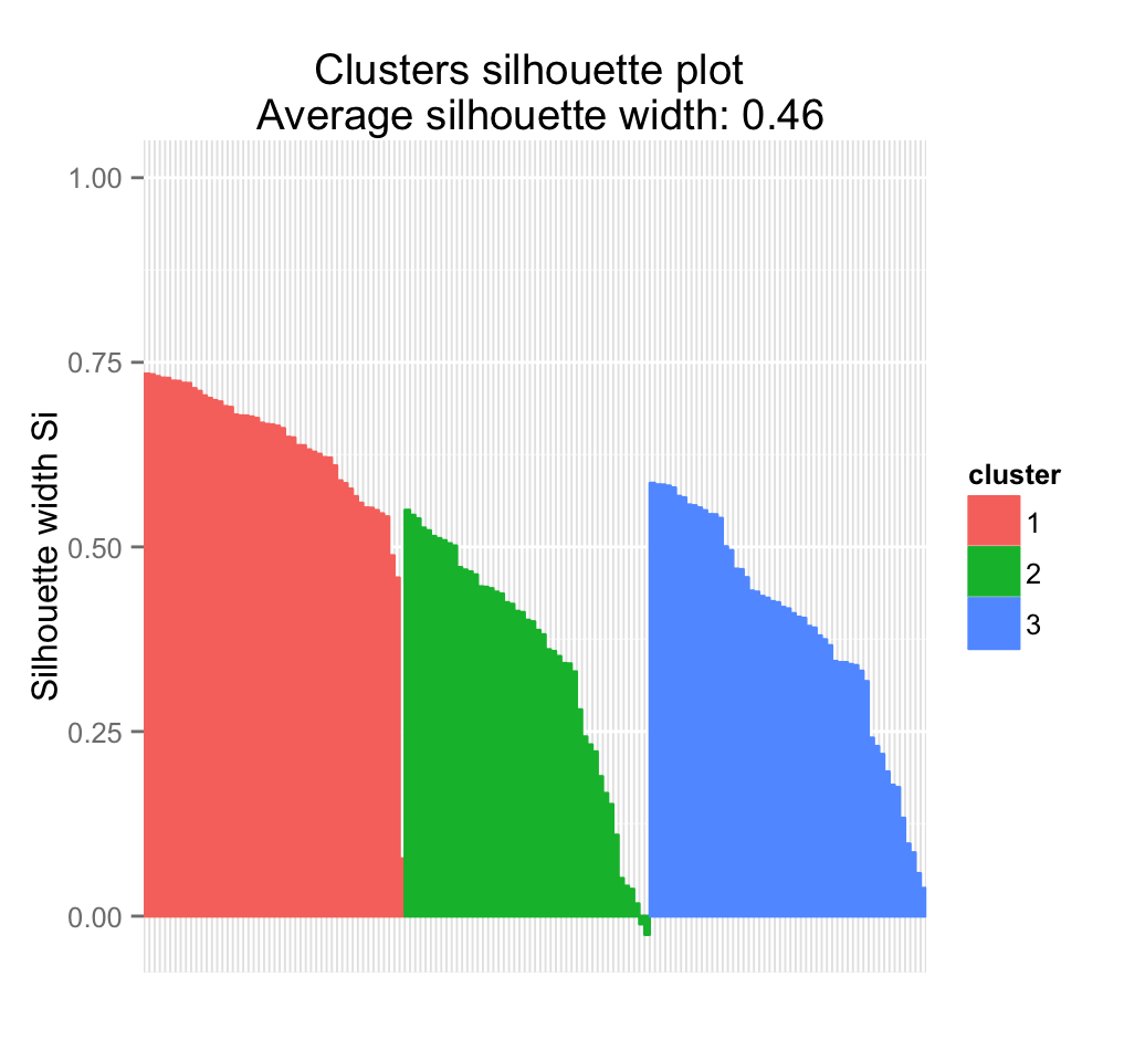
# Change the theme and color
fviz_silhouette(km.res, print.summary = FALSE) +
scale_fill_brewer(palette = "Dark2") +
scale_color_brewer(palette = "Dark2") +
theme_minimal()+
theme(axis.text.x = element_blank(), axis.ticks.x = element_blank())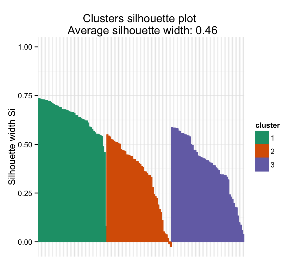
Silhouette information can be extracted as follow:
# Silhouette information
silinfo <- km.res$silinfo
names(silinfo)## [1] "widths" "clus.avg.widths" "avg.width"# Silhouette widths of each observation
head(silinfo$widths[, 1:3], 10)## cluster neighbor sil_width
## 1 1 3 0.7341949
## 41 1 3 0.7333345
## 8 1 3 0.7308169
## 18 1 3 0.7287522
## 5 1 3 0.7284741
## 40 1 3 0.7247047
## 38 1 3 0.7244191
## 12 1 3 0.7217939
## 28 1 3 0.7215103
## 29 1 3 0.7145192# Average silhouette width of each cluster
silinfo$clus.avg.widths## [1] 0.6363162 0.3473922 0.3933772# The total average (mean of all individual silhouette widths)
silinfo$avg.width## [1] 0.4599482# The size of each clusters
km.res$size## [1] 50 47 535.1.5 Silhouette plot for PAM clustering
fviz_silhouette(pam.res)## cluster size ave.sil.width
## 1 1 50 0.63
## 2 2 45 0.35
## 3 3 55 0.38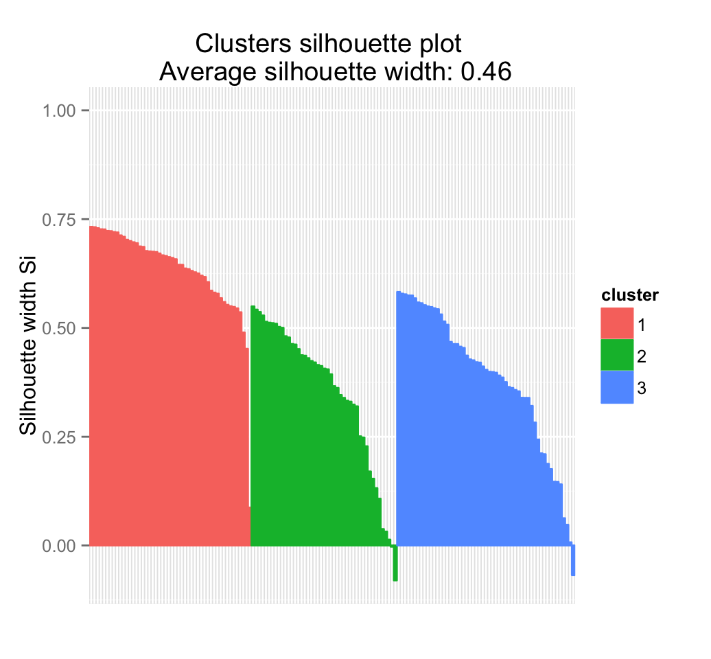
5.1.6 Silhouette plot for hierarchical clustering
fviz_silhouette(res.hc)## cluster size ave.sil.width
## 1 1 49 0.75
## 2 2 75 0.37
## 3 3 26 0.51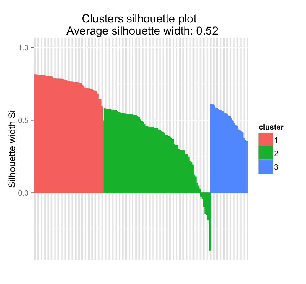
5.1.7 Samples with a negative silhouette coefficient
It can be seen that several samples have a negative silhouette coefficient in the hierarchical clustering. This means that they are not in the right cluster.
We can find the name of these samples and determine the clusters they are closer (neighbor cluster), as follow:
# Silhouette width of observation
sil <- res.hc$silinfo$widths[, 1:3]
# Objects with negative silhouette
neg_sil_index <- which(sil[, 'sil_width'] < 0)
sil[neg_sil_index, , drop = FALSE]## cluster neighbor sil_width
## 51 2 3 -0.02848264
## 148 2 3 -0.03799687
## 129 2 3 -0.09622863
## 111 2 3 -0.14461589
## 109 2 3 -0.14991556
## 133 2 3 -0.18730218
## 42 2 1 -0.395150105.2 Dunn index
5.2.1 Concept and algorithm
Dunn index is another internal clustering validation measure which can be computed as follow:
- For each cluster, compute the distance between each of the objects in the cluster and the objects in the other clusters
Use the minimum of this pairwise distance as the inter-cluster separation (min.separation)
- For each cluster, compute the distance between the objects in the same cluster.
Use the maximal intra-cluster distance (i.e maximum diameter) as the intra-cluster compactness
Calculate Dunn index (D) as follow:
\[ D = \frac{min.separation}{max.diameter} \]
If the data set contains compact and well-separated clusters, the diameter of the clusters is expected to be small and the distance between the clusters is expected to be large. Thus, Dunn index should be maximized.
5.2.2 R function for computing Dunn index
The function cluster.stats() [in fpc package] and the function NbClust() [in NbClust package] can be used to compute Dunn index and many other indices.
The function cluster.stats() is described in the next section.
5.3 Clustering validation statistics
In this section, we’ll describe the R function cluster.stats() [in fpc package] for computing a number of distance based statistics which can be used either for cluster validation, comparison between clustering and decision about the number of clusters.
The simplified format is:
cluster.stats(d = NULL, clustering, al.clustering = NULL)- d: a distance object between cases as generated by the dist() function
- clustering: vector containing the cluster number of each observation
- alt.clustering: vector such as for clustering, indicating an alternative clustering
The function cluster.stats() returns a list containing many components useful for analyzing the intrinsic characteristics of a clustering:
- cluster.number: number of clusters
- cluster.size: vector containing the number of points in each cluster
- average.distance, median.distance: vector containing the cluster-wise within average/median distances
- average.between: average distance between clusters. We want it to be as large as possible
- average.within: average distance within clusters. We want it to be as small as possible
- clus.avg.silwidths: vector of cluster average silhouette widths. Recall that, the silhouette width is also an estimate of the average distance between clusters. Its value is comprised between 1 and -1 with a value of 1 indicating a very good cluster.
- within.cluster.ss: a generalization of the within clusters sum of squares (k-means objective function), which is obtained if d is a Euclidean distance matrix.
- dunn, dunn2: Dunn index
- corrected.rand, vi: Two indexes to assess the similarity of two clustering: the corrected Rand index and Meila’s VI
All the above elements can be used to evaluate the internal quality of clustering.
In the following sections, we’ll compute the clustering quality statistics for k-means, pam and hierarchical clustering. Look at the within.cluster.ss (within clusters sum of squares), the average.within (average distance within clusters) and clus.avg.silwidths (vector of cluster average silhouette widths).
5.3.0.1 Cluster statistics for k-means clustering
library(fpc)
# Compute pairwise-distance matrices
dd <- dist(iris.scaled, method ="euclidean")
# Statistics for k-means clustering
km_stats <- cluster.stats(dd, km.res$cluster)
# (k-means) within clusters sum of squares
km_stats$within.cluster.ss## [1] 138.8884# (k-means) cluster average silhouette widths
km_stats$clus.avg.silwidths## 1 2 3
## 0.6363162 0.3473922 0.3933772# Display all statistics
km_stats## $n
## [1] 150
##
## $cluster.number
## [1] 3
##
## $cluster.size
## [1] 50 47 53
##
## $min.cluster.size
## [1] 47
##
## $noisen
## [1] 0
##
## $diameter
## [1] 5.034198 3.343671 2.922371
##
## $average.distance
## [1] 1.175155 1.307716 1.197061
##
## $median.distance
## [1] 0.9884177 1.2383531 1.1559887
##
## $separation
## [1] 1.5533592 0.1333894 0.1333894
##
## $average.toother
## [1] 3.647912 3.081212 2.674298
##
## $separation.matrix
## [,1] [,2] [,3]
## [1,] 0.000000 2.4150235 1.5533592
## [2,] 2.415024 0.0000000 0.1333894
## [3,] 1.553359 0.1333894 0.0000000
##
## $ave.between.matrix
## [,1] [,2] [,3]
## [1,] 0.000000 4.129179 3.221129
## [2,] 4.129179 0.000000 2.092563
## [3,] 3.221129 2.092563 0.000000
##
## $average.between
## [1] 3.130708
##
## $average.within
## [1] 1.222246
##
## $n.between
## [1] 7491
##
## $n.within
## [1] 3684
##
## $max.diameter
## [1] 5.034198
##
## $min.separation
## [1] 0.1333894
##
## $within.cluster.ss
## [1] 138.8884
##
## $clus.avg.silwidths
##         1         2         3
## 0.6363162 0.3473922 0.3933772
##
## $avg.silwidth
## [1] 0.4599482
##
## $g2
## NULL
##
## $g3
## NULL
##
## $pearsongamma
## [1] 0.679696
##
## $dunn
## [1] 0.02649665
##
## $dunn2
## [1] 1.600166
##
## $entropy
## [1] 1.097412
##
## $wb.ratio
## [1] 0.3904057
##
## $ch
## [1] 241.9044
##
## $cwidegap
## [1] 1.3892251 0.9432249 0.7824508
##
## $widestgap
## [1] 1.389225
##
## $sindex
## [1] 0.3524812
##
## $corrected.rand
## NULL
##
## $vi
## NULLRead the documentation of cluster.stats() for details about all the available indices.
The same statistics can be computed for pam clustering and hierarchical clustering.
5.3.0.2 Cluster statistics for PAM clustering
# Statistics for pam clustering
pam_stats <- cluster.stats(dd,  pam.res$cluster)
# (pam) within clusters sum of squares
pam_stats$within.cluster.ss
## [1] 140.2856# (pam) cluster average silhouette widths
pam_stats$clus.avg.silwidths## 1 2 3
## 0.6346397 0.3496332 0.38238175.3.0.3 Cluster statistics for hierarchical clustering
# Statistics for hierarchical clustering
hc_stats <- cluster.stats(dd,  res.hc$cluster)
# (HCLUST) within clusters sum of squares
hc_stats$within.cluster.ss
## [1] 152.7107# (HCLUST) cluster average silhouette widths
hc_stats$clus.avg.silwidths## 1 2 3
## 0.6688130 0.3154184 0.44881976 External clustering validation
The aim is to compare the identified clusters (by k-means, pam or hierarchical clustering) to a reference.
To compare two cluster solutions, use the cluster.stats() function as follow:
res.stat <- cluster.stats(d, solution1$cluster, solution2$cluster)Among the values returned by the function cluster.stats(), there are two indexes to assess the similarity of two clustering, namely the corrected Rand index and Meila’s VI.
We know that the iris data contains exactly 3 groups of species.
Does the K-means clustering matches with the true structure of the data?
We can use the function cluster.stats() to answer to this question.
A cross-tabulation can be computed as follow:
table(iris$Species, km.res$cluster)##
## 1 2 3
## setosa 50 0 0
## versicolor 0 11 39
## virginica 0 36 14It can be seen that:
- All setosa species (n = 50) has been classified in cluster 1
- A large number of versicor species (n = 39 ) has been classified in cluster 3. Some of them ( n = 11) have been classified in cluster 2.
- A large number of virginica species (n = 36 ) has been classified in cluster 2. Some of them (n = 14) have been classified in cluster 3.
It’s possible to quantify the agreement between Species and k-means clusters using either the corrected Rand index and Meila’s VI provided as follow:
library("fpc")
# Compute cluster stats
species <- as.numeric(iris$Species)
clust_stats <- cluster.stats(d = dist(iris.scaled),
                             species, km.res$cluster)
# Corrected Rand index
clust_stats$corrected.rand
## [1] 0.6201352# VI
clust_stats$vi## [1] 0.7477749The corrected Rand index provides a measure for assessing the similarity between two partitions, adjusted for chance. Its range is -1 (no agreement) to 1 (perfect agreement). Agreement between the specie types and the cluster solution is 0.62 using Rand index and 0.748 using Meila’s VI
The same analysis can be computed for both pam and hierarchical clustering:
# Agreement between species and pam clusters
table(iris$Species, pam.res$cluster)
##
## 1 2 3
## setosa 50 0 0
## versicolor 0 9 41
## virginica 0 36 14cluster.stats(d = dist(iris.scaled),
species, pam.res$cluster)$vi## [1] 0.7129034# Agreement between species and HC clusters
table(iris$Species, res.hc$cluster)##
## 1 2 3
## setosa 49 1 0
## versicolor 0 50 0
## virginica 0 24 26cluster.stats(d = dist(iris.scaled),
species, res.hc$cluster)$vi## [1] 0.6097098External clustering validation, can be used to select suitable clustering algorithm for a given dataset.
7 Infos
This analysis has been performed using R software (ver. 3.2.1)
- Malika Charrad, Nadia Ghazzali, Veronique Boiteau, Azam Niknafs (2014). NbClust: An R Package for Determining the Relevant Number of Clusters in a Data Set. Journal of Statistical Software, 61(6), 1-36. URL http://www.jstatsoft.org/v61/i06/.
- Theodoridis S, Koutroubas K (2008). Pattern Recognition. 4th edition. Academic Press.
Show me some love with the like buttons below... Thank you and please don't forget to share and comment below!!
Montrez-moi un peu d'amour avec les like ci-dessous ... Merci et n'oubliez pas, s'il vous plaît, de partager et de commenter ci-dessous!
Recommended for You!
Recommended for you
This section contains the best data science and self-development resources to help you on your path.
Books - Data Science
Our Books
- Practical Guide to Cluster Analysis in R by A. Kassambara (Datanovia)
- Practical Guide To Principal Component Methods in R by A. Kassambara (Datanovia)
- Machine Learning Essentials: Practical Guide in R by A. Kassambara (Datanovia)
- R Graphics Essentials for Great Data Visualization by A. Kassambara (Datanovia)
- GGPlot2 Essentials for Great Data Visualization in R by A. Kassambara (Datanovia)
- Network Analysis and Visualization in R by A. Kassambara (Datanovia)
- Practical Statistics in R for Comparing Groups: Numerical Variables by A. Kassambara (Datanovia)
- Inter-Rater Reliability Essentials: Practical Guide in R by A. Kassambara (Datanovia)
Others
- R for Data Science: Import, Tidy, Transform, Visualize, and Model Data by Hadley Wickham & Garrett Grolemund
- Hands-On Machine Learning with Scikit-Learn, Keras, and TensorFlow: Concepts, Tools, and Techniques to Build Intelligent Systems by Aurelien Géron
- Practical Statistics for Data Scientists: 50 Essential Concepts by Peter Bruce & Andrew Bruce
- Hands-On Programming with R: Write Your Own Functions And Simulations by Garrett Grolemund & Hadley Wickham
- An Introduction to Statistical Learning: with Applications in R by Gareth James et al.
- Deep Learning with R by François Chollet & J.J. Allaire
- Deep Learning with Python by François Chollet
Click to follow us on Facebook :
Comment this article by clicking on "Discussion" button (top-right position of this page)


