


DBSCAN: density-based clustering for discovering clusters in large datasets with noise - Unsupervised Machine Learning
1 Concepts of density-based clustering
Partitioning methods (K-means, PAM clustering) and hierarchical clustering are suitable for finding spherical-shaped clusters or convex clusters. In other words, they work well for compact and well separated clusters. Moreover, they are also severely affected by the presence of noise and outliers in the data.
Unfortunately, real life data can contain: i) clusters of arbitrary shape such as those shown in the figure below (oval, linear and “S” shape clusters); ii) many outliers and noise.
The figure below shows a dataset containing nonconvex clusters and outliers/noises. The simulated dataset multishapes [in factoextra package] is used.

The plot above contains 5 clusters and outliers, including:
- 2 ovales clusters
- 2 linear clusters
- 1 compact cluster
Given such data, k-means algorithm has difficulties for identifying theses clusters with arbitrary shape. To illustrate this situation, the following R code computes K-means algorithm on the dataset multishapes [in factoextra package]. The function fviz_cluster() [in factoextra] is used to visualize the clusters.
The latest version of factoextra can be installed using the following R code:
if(!require(devtools)) install.packages("devtools")
devtools::install_github("kassambara/factoextra")
Compute and visualize k-means clustering using the dataset multishapes:
library(factoextra)
data("multishapes")
df <- multishapes[, 1:2]
set.seed(123)
km.res <- kmeans(df, 5, nstart = 25)
fviz_cluster(km.res, df, frame = FALSE, geom = "point")
We know there are 5 five clusters in the data, but it can be seen that k-means method inaccurately identify the 5 clusters.
This chapter describes DBSCAN, a density-based clustering algorithm, introduced in Ester et al. 1996, which can be used to identify clusters of any shape in data set containing noise and outliers. DBSCAN stands for Density-Based Spatial Clustering and Application with Noise.
The advantages of DBSCAN are:
- Unlike K-means, DBSCAN does not require the user to specify the number of clusters to be generated
- DBSCAN can find any shape of clusters. The cluster doesn’t have to be circular.
- DBSCAN can identify outliers
The basic idea behind density-based clustering approach is derived from a human intuitive clustering method. For instance, by looking at the figure below, one can easily identify four clusters along with several points of noise, because of the differences in the density of points.
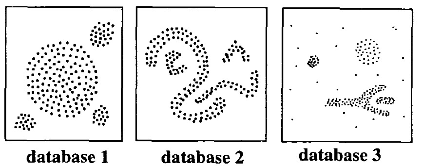 (From Ester et al. 1996)
As illustrated in the figure above, clusters are dense regions in the data space, separated by regions of lower density of points. In other words, the density of points in a cluster is considerably higher than the density of points outside the cluster (“areas of noise”).
DBSCAN is based on this intuitive notion of “clusters” and “noise”. The key idea is that for each point of a cluster, the neighborhood of a given radius has to contain at least a minimum number of points.
2 Algorithm of DBSCAN
The goal is to identify dense regions, which can be measured by the number of objects close to a given point.
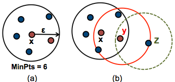
Two important parameters are required for DBSCAN: epsilon (“eps”) and minimum points (“MinPts”). The parameter eps defines the radius of neighborhood around a point x. It’s called called the \(\epsilon\)-neighborhood of x. The parameter MinPts is the minimum number of neighbors within “eps” radius.
Any point x in the dataset, with a neighbor count greater than or equal to MinPts, is marked as a core point. We say that x is border point, if the number of its neighbors is less than MinPts, but it belongs to the \(\epsilon\)-neighborhood of some core point z. Finally, if a point is neither a core nor a border point, then it is called a noise point or an outlier.
The figure below shows the different types of points (core, border and outlier points) using MinPts = 6. Here x is a core point because \(neighbours_\epsilon(x) = 6\), y is a border point because \(neighbours_\epsilon(y) < MinPts\), but it belongs to the \(\epsilon\)-neighborhood of the core point x. Finally, z is a noise point.
We define 3 terms, required for understanding the DBSCAN algorithm:
- Direct density reachable: A point “A” is directly density reachable from another point “B” if: i) “A” is in the \(\epsilon\)-neighborhood of “B” and ii) “B” is a core point.
- Density reachable: A point “A” is density reachable from “B” if there are a set of core points leading from “B” to “A.
- Density connected: Two points “A” and “B” are density connected if there are a core point “C”, such that both “A” and “B” are density reachable from “C”.
A density-based cluster is defined as a group of density connected points. The algorithm of density-based clustering (DBSCAN) works as follow:
The algorithm of density-based clustering works as follow:
- For each point \(x_i\), compute the distance between \(x_i\) and the other points. Finds all neighbor points within distance eps of the starting point (\(x_i\)). Each point, with a neighbor count greater than or equal to MinPts, is marked as core point or visited.
- For each core point, if it’s not already assigned to a cluster, create a new cluster. Find recursively all its density connected points and assign them to the same cluster as the core point.
- Iterate through the remaining unvisited points in the dataset.
3 R packages for computing DBSCAN
Three R packages are used in this article:
- fpc and dbscan for computing density-based clustering
- factoextra for visualizing clusters
The R packages fpc and dbscan can be installed as follow:
install.packages("fpc")
install.packages("dbscan")
4 R functions for DBSCAN
The function dbscan() [in fpc package] or dbscan() [in dbscan package] can be used.
As the name of DBSCAN functions is the same in the two packages, we’ll explicitly use them as follow: fpc::dbscan() and dbscan::dbscan().
In the following examples, we’ll use fpc package. A simplified format of the function is:
dbscan(data, eps, MinPts = 5, scale = FALSE,
method = c("hybrid", "raw", "dist"))- data: data matrix, data frame or dissimilarity matrix (dist-object). Specify method = “dist” if the data should be interpreted as dissimilarity matrix or object. Otherwise Euclidean distances will be used.
- eps: Reachability maximum distance
- MinPts: Reachability minimum number of points
- scale: If TRUE, the data will be scaled
- method: Possible values are:
- dist: Treats the data as distance matrix
- raw: Treats the data as raw data
- hybrid: Expect also raw data, but calculates partial distance matrices
Recall that, DBSCAN clusters require a minimum number of points (MinPts) within a maximum distance (eps) around one of its members (the seed).
Any point within eps around any point which satisfies the seed condition is a cluster member (recursively).
- Some points may not belong to any clusters (noise).
In the following examples, we’ll use the simulated multishapes data [in factoextra package]:
# Load the data
# Make sure that the package factoextra is installed
data("multishapes", package = "factoextra")
df <- multishapes[, 1:2]
The function dbscan() can be used as follow:
library("fpc")
# Compute DBSCAN using fpc package
set.seed(123)
db <- fpc::dbscan(df, eps = 0.15, MinPts = 5)
# Plot DBSCAN results
plot(db, df, main = "DBSCAN", frame = FALSE)
Note that, the function plot.dbscan() uses different point symbols for core points (i.e, seed points) and border points. Black points correspond to outliers. You can play with eps and MinPts for changing cluster configurations.
It can be seen that DBSCAN performs better for these data sets and can identify the correct set of clusters compared to k-means algorithms.
It’s also possible to draw the plot above using the function fviz_cluster() [ in factoextra package]:
library("factoextra")
fviz_cluster(db, df, stand = FALSE, frame = FALSE, geom = "point")
The result of fpc::dbscan() function can be displayed as follow:
# Print DBSCAN
print(db)
## dbscan Pts=1100 MinPts=5 eps=0.15
## 0 1 2 3 4 5
## border 31 24 1 5 7 1
## seed 0 386 404 99 92 50
## total 31 410 405 104 99 51In the table above, column names are cluster number. Cluster 0 corresponds to outliers (black points in the DBSCAN plot).
# Cluster membership. Noise/outlier observations are coded as 0
# A random subset is shown
db$cluster[sample(1:1089, 50)]
## [1] 1 3 2 4 3 1 2 4 2 2 2 2 2 2 1 4 1 1 1 0 4 2 2 5 2 2 2 2 1 1 0 4 2 3 1
## [36] 2 2 1 1 1 1 2 2 1 1 1 3 2 1 3The function print.dbscan() shows a statistic of the number of points belonging to the clusters that are seeds and border points.
DBSCAN algorithm requires users to specify the optimal eps values and the parameter MinPts. In the R code above, we used eps = 0.15 and MinPts = 5. One limitation of DBSCAN is that it is sensitive to the choice of \(\epsilon\), in particular if clusters have different densities. If \(\epsilon\) is too small, sparser clusters will be defined as noise. If \(\epsilon\) is too large, denser clusters may be merged together. This implies that, if there are clusters with different local densities, then a single \(\epsilon\) value may not suffice.
A natural question is:
How to define the optimal value of eps?
5 Method for determining the optimal eps value
The method proposed here consists of computing the he k-nearest neighbor distances in a matrix of points.
The idea is to calculate, the average of the distances of every point to its k nearest neighbors. The value of k will be specified by the user and corresponds to MinPts.
Next, these k-distances are plotted in an ascending order. The aim is to determine the “knee”, which corresponds to the optimal eps parameter.
A knee corresponds to a threshold where a sharp change occurs along the k-distance curve.
The function kNNdistplot() [in dbscan package] can be used to draw the k-distance plot:
dbscan::kNNdistplot(df, k =  5)
abline(h = 0.15, lty = 2)
It can be seen that the optimal eps value is around a distance of 0.15.
6 Cluster predictions with DBSCAN algorithm
The function predict.dbscan(object, data, newdata) [in fpc package] can be used to predict the clusters for the points in newdata. For more details, read the documentation (?predict.dbscan).
7 Application of DBSCAN on a real data
The iris dataset is used:
# Load the data
data("iris")
iris <- as.matrix(iris[, 1:4])
The optimal value of “eps” parameter can be determined as follow:
dbscan::kNNdistplot(iris, k =  4)
abline(h = 0.4, lty = 2)
Compute DBSCAN using fpc::dbscan() and dbscan::dbscan(). Make sure that the 2 packages are installed:
set.seed(123)
# fpc package
res.fpc <- fpc::dbscan(iris, eps = 0.4, MinPts = 4)
# dbscan package
res.db <- dbscan::dbscan(iris, 0.4, 4)- The result of the function fpc::dbscan() provides an object of class ‘dbscan’ containing the following components:
- cluster: integer vector coding cluster membership with noise observations (singletons) coded as 0
- isseed: logical vector indicating whether a point is a seed (not border, not noise)
- eps: parameter eps
- MinPts: parameter MinPts
- The result of the function dbscan::dbscan() is an integer vector with cluster assignments. Zero indicates noise points.
Note that the function dbscan:dbscan() is a fast re-implementation of DBSCAN algorithm. The implementation is significantly faster and can work with larger data sets than the function fpc:dbscan().
Make sure that both version produce the same results:
all(res.fpc$cluster == res.db)## [1] TRUEThe result can be visualized as follow:
fviz_cluster(res.fpc, iris, geom = "point")
Black points are outliers.
8 Infos
This analysis has been performed using R software (ver. 3.2.1)
- Martin Ester, Hans-Peter Kriegel, Joerg Sander, Xiaowei Xu (1996). A Density-Based Algorithm for Discovering Clusters in Large Spatial Databases with Noise. Institute for Computer Science, University of Munich. Proceedings of 2nd International Conference on Knowledge Discovery and Data Mining (KDD-96)
Show me some love with the like buttons below... Thank you and please don't forget to share and comment below!!
Montrez-moi un peu d'amour avec les like ci-dessous ... Merci et n'oubliez pas, s'il vous plaît, de partager et de commenter ci-dessous!
Recommended for You!


Recommended for you
This section contains the best data science and self-development resources to help you on your path.
Books - Data Science
Our Books
- Practical Guide to Cluster Analysis in R by A. Kassambara (Datanovia)
- Practical Guide To Principal Component Methods in R by A. Kassambara (Datanovia)
- Machine Learning Essentials: Practical Guide in R by A. Kassambara (Datanovia)
- R Graphics Essentials for Great Data Visualization by A. Kassambara (Datanovia)
- GGPlot2 Essentials for Great Data Visualization in R by A. Kassambara (Datanovia)
- Network Analysis and Visualization in R by A. Kassambara (Datanovia)
- Practical Statistics in R for Comparing Groups: Numerical Variables by A. Kassambara (Datanovia)
- Inter-Rater Reliability Essentials: Practical Guide in R by A. Kassambara (Datanovia)
Others
- R for Data Science: Import, Tidy, Transform, Visualize, and Model Data by Hadley Wickham & Garrett Grolemund
- Hands-On Machine Learning with Scikit-Learn, Keras, and TensorFlow: Concepts, Tools, and Techniques to Build Intelligent Systems by Aurelien Géron
- Practical Statistics for Data Scientists: 50 Essential Concepts by Peter Bruce & Andrew Bruce
- Hands-On Programming with R: Write Your Own Functions And Simulations by Garrett Grolemund & Hadley Wickham
- An Introduction to Statistical Learning: with Applications in R by Gareth James et al.
- Deep Learning with R by François Chollet & J.J. Allaire
- Deep Learning with Python by François Chollet
Click to follow us on Facebook :
Comment this article by clicking on "Discussion" button (top-right position of this page)