


Introduction to RNA sequencing
This analysis was performed using R (ver. 3.1.0).Principle
RNA extraction conversion to cDNA fragmentation sequencing this gives reads map to the genome.
We want to know, genes differentially expressed between 2 samples, 1 and 2. Each sample has a series of reads, and we can just simply find how many map by aligning each sample to the genome. In the cartoon down below, we see that sample 1 has more gene expression for gene A and B, than sample 2, and you can do statistics on that.
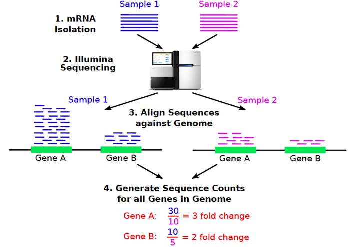 (source : Thomas Girke, Analysis of RNA-Seq Data with R/Bioconductor, December 14, 2013)
After counting the number of reads which map to the reference genome, we have a big matrix with samples on the columns and gene on the rows. You can apply very similar approaches to the ones that we described earlier for microarray data. However most of the approaches that are currently used to analyze read counts, model the counts with Poisson or negative binomial. Two widely used methods that do this are edgeR and DESeq.
Genes aren’t just a piece of the genome
For humans, genes conatin exons and introns. So the sequence of the RNA transcript aren’t exactly represented on the genome, and in this cartoon we see what happens.
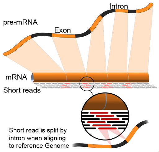
Yellow color is exons and black color is intron. When RNA is transcribed, these introns are spliced out, and we create an RNA transcript that only contains the exons. This means that, we have these regions, called junctions.
For the reads which come from junctions: one part of it maps to one exon and the other half maps to the other exon.
A second complication is that the same gene can have many different transcripts. So one of the new possibilities that RNA-seq opens up, is the ability to measure these different transcripts. You might have a sample where, even though the gene expression for a given gene is the same in the two samples of the two populations, in one population you see an over-representation of one of the transcripts compared to the other.
While we have approaches like edgeR, DESeq, and DEXSeq that basically count each gene or each exon and quantifies the amount, we also have techniques that try to determine from the reads what transcripts are present. Examples of these methods are Trinity Oases, Cufflinks, and Scripture.
Alignement and read counting
You have to map the reads to the genome, taking into account that some of these reads might be split between two distant parts of the genome. There’s a gap. After alignment, we know which read comes from which exon and which reads come from which junction. So example of software that does that is TopHat, GSNAP, MapSplice, STAR.
The output of alignment softwares is bam file. To quantify how much of each transcript we have, software like Cufflinks can be used for reads counting.
You can also use this information to create the gene count tables. You can basically count all the reads that fall into a gene, regardless of what transcript they come from.
You could also do counts for at the exon level. This creates the table where you can then do things like differential expression. You have a table of counts for either exons or genes on the rows, and samples on the columns.
Licence
References
Show me some love with the like buttons below... Thank you and please don't forget to share and comment below!!
Montrez-moi un peu d'amour avec les like ci-dessous ... Merci et n'oubliez pas, s'il vous plaît, de partager et de commenter ci-dessous!
Recommended for You!


Recommended for you
This section contains the best data science and self-development resources to help you on your path.
Books - Data Science
Our Books
- Practical Guide to Cluster Analysis in R by A. Kassambara (Datanovia)
- Practical Guide To Principal Component Methods in R by A. Kassambara (Datanovia)
- Machine Learning Essentials: Practical Guide in R by A. Kassambara (Datanovia)
- R Graphics Essentials for Great Data Visualization by A. Kassambara (Datanovia)
- GGPlot2 Essentials for Great Data Visualization in R by A. Kassambara (Datanovia)
- Network Analysis and Visualization in R by A. Kassambara (Datanovia)
- Practical Statistics in R for Comparing Groups: Numerical Variables by A. Kassambara (Datanovia)
- Inter-Rater Reliability Essentials: Practical Guide in R by A. Kassambara (Datanovia)
Others
- R for Data Science: Import, Tidy, Transform, Visualize, and Model Data by Hadley Wickham & Garrett Grolemund
- Hands-On Machine Learning with Scikit-Learn, Keras, and TensorFlow: Concepts, Tools, and Techniques to Build Intelligent Systems by Aurelien Géron
- Practical Statistics for Data Scientists: 50 Essential Concepts by Peter Bruce & Andrew Bruce
- Hands-On Programming with R: Write Your Own Functions And Simulations by Garrett Grolemund & Hadley Wickham
- An Introduction to Statistical Learning: with Applications in R by Gareth James et al.
- Deep Learning with R by François Chollet & J.J. Allaire
- Deep Learning with Python by François Chollet
Click to follow us on Facebook :
Comment this article by clicking on "Discussion" button (top-right position of this page)