


ggplot2 - Easy Way to Mix Multiple Graphs on The Same Page
To arrange multiple ggplot2 graphs on the same page, the standard R functions - par() and layout() - cannot be used.
The basic solution is to use the gridExtra R package, which comes with the following functions:
- grid.arrange() and arrangeGrob() to arrange multiple ggplots on one page
- marrangeGrob() for arranging multiple ggplots over multiple pages.
However, these functions makes no attempt at aligning the plot panels; instead, the plots are simply placed into the grid as they are, and so the axes are not aligned.
If axis alignment is required, you can switch to the cowplot package, which include the function plot_grid() with the argument align. However, the cowplot package doesn’t contain any solution for multi-pages layout. Therefore, we provide the function ggarrange() [in ggpubr], a wrapper around the plot_grid() function, to arrange multiple ggplots over multiple pages. It can also create a common unique legend for multiple plots.
This article will show you, step by step, how to combine multiple ggplots on the same page, as well as, over multiple pages, using helper functions available in the following R package: ggpubr R package, cowplot and gridExtra. We’ll also describe how to export the arranged plots to a file.
Related articles:
Contents:
- Prerequisites
- Create some plots
- Arrange on one page
- Annotate the arranged figure
- Align plot panels
- Change column/row span of a plot
- Use common legend for combined ggplots
- Scatter plot with marginal density plots
- Mix table, text and ggplot2 graphs
- Insert a graphical element inside a ggplot
- Arrange over multiple pages
- Nested layout with ggarrange()
- Export plots
- Acknoweledgment
Prerequisites
Required R package
You need to install the R package ggpubr (version >= 0.1.3), to easily create ggplot2-based publication ready plots.
We recommend to install the latest developmental version from GitHub as follow:
if(!require(devtools)) install.packages("devtools")
devtools::install_github("kassambara/ggpubr")
If installation from Github failed, then try to install from CRAN as follow:
install.packages("ggpubr")Note that, the installation of ggpubr will automatically install the gridExtra and the cowplot package; so you don’t need to re-install them.
Load ggpubr:
library(ggpubr)Demo data sets
Data: ToothGrowth and mtcars data sets.
# ToothGrowth
data("ToothGrowth")
head(ToothGrowth)
## len supp dose
## 1 4.2 VC 0.5
## 2 11.5 VC 0.5
## 3 7.3 VC 0.5
## 4 5.8 VC 0.5
## 5 6.4 VC 0.5
## 6 10.0 VC 0.5# mtcars
data("mtcars")
mtcars$name <- rownames(mtcars)
mtcars$cyl <- as.factor(mtcars$cyl)
head(mtcars[, c("name", "wt", "mpg", "cyl")])## name wt mpg cyl
## Mazda RX4 Mazda RX4 2.62 21.0 6
## Mazda RX4 Wag Mazda RX4 Wag 2.88 21.0 6
## Datsun 710 Datsun 710 2.32 22.8 4
## Hornet 4 Drive Hornet 4 Drive 3.21 21.4 6
## Hornet Sportabout Hornet Sportabout 3.44 18.7 8
## Valiant Valiant 3.46 18.1 6Create some plots
Here, we’ll use ggplot2-based plotting functions available in ggpubr. You can use any ggplot2 functions to create the plots that you want for arranging them later.
We’ll start by creating 4 different plots:
- Box plots and dot plots using the ToothGrowth data set
- Bar plots and scatter plots using the mtcars data set
You’ll learn how to combine these plots in the next sections using specific functions.
- Create a box plot and a dot plot:
# Box plot (bp)
bxp <- ggboxplot(ToothGrowth, x = "dose", y = "len",
color = "dose", palette = "jco")
bxp
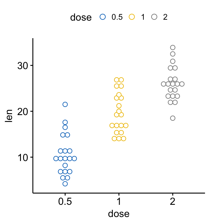
# Dot plot (dp)
dp <- ggdotplot(ToothGrowth, x = "dose", y = "len",
color = "dose", palette = "jco", binwidth = 1)
dp
- Create an ordered bar plot and a scatter plot:
Create ordered bar plots. Change the fill color by the grouping variable “cyl”. Sorting will be done globally, but not by groups.
# Bar plot (bp)
bp <- ggbarplot(mtcars, x = "name", y = "mpg",
          fill = "cyl",               # change fill color by cyl
          color = "white",            # Set bar border colors to white
          palette = "jco",            # jco journal color palett. see ?ggpar
          sort.val = "asc",           # Sort the value in ascending order
          sort.by.groups = TRUE,      # Sort inside each group
          x.text.angle = 90           # Rotate vertically x axis texts
          )
bp + font("x.text", size = 8)
# Scatter plots (sp)
sp <- ggscatter(mtcars, x = "wt", y = "mpg",
                add = "reg.line",               # Add regression line
                conf.int = TRUE,                # Add confidence interval
                color = "cyl", palette = "jco", # Color by groups "cyl"
                shape = "cyl"                   # Change point shape by groups "cyl"
                )+
  stat_cor(aes(color = cyl), label.x = 3)       # Add correlation coefficient
sp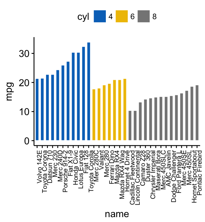

Arrange on one page
To arrange multiple ggplots on one single page, we’ll use the function ggarrange()[in ggpubr], which is a wrapper around the function plot_grid() [in cowplot package]. Compared to the standard function plot_grid(), ggarange() can arrange multiple ggplots over multiple pages.
ggarrange(bxp, dp, bp + rremove("x.text"),
          labels = c("A", "B", "C"),
          ncol = 2, nrow = 2)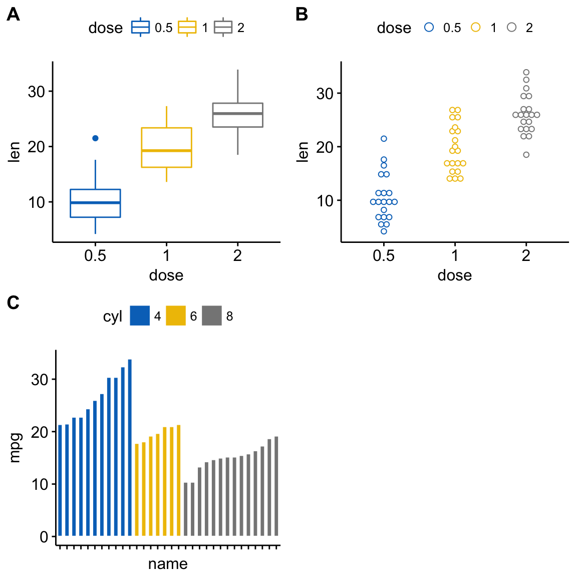
Alternatively, you can also use the function plot_grid() [in cowplot]:
library("cowplot")
plot_grid(bxp, dp, bp + rremove("x.text"),
          labels = c("A", "B", "C"),
          ncol = 2, nrow = 2)
or, the function grid.arrange() [in gridExtra]:
library("gridExtra")
grid.arrange(bxp, dp, bp + rremove("x.text"),
             ncol = 2, nrow = 2)
Annotate the arranged figure
R function: annotate_figure() [in ggpubr].
figure <- ggarrange(sp, bp + font("x.text", size = 10),
                    ncol = 1, nrow = 2)
annotate_figure(figure,
                top = text_grob("Visualizing mpg", color = "red", face = "bold", size = 14),
                bottom = text_grob("Data source: \n mtcars data set", color = "blue",
                                   hjust = 1, x = 1, face = "italic", size = 10),
                left = text_grob("Figure arranged using ggpubr", color = "green", rot = 90),
                right = "I'm done, thanks :-)!",
                fig.lab = "Figure 1", fig.lab.face = "bold"
                )
Note that, the function annotate_figure() supports any ggplots.
Align plot panels
A real use case is, for example, when plotting survival curves with the risk table placed under the main plot.
To illustrate this case, we’ll use the survminer package. First, install it using install.packages(“survminer”), then type this:
# Fit survival curves
library(survival)
fit <- survfit( Surv(time, status) ~ adhere, data = colon )
# Plot survival curves
library(survminer)
ggsurv <- ggsurvplot(fit, data = colon,
                     palette = "jco",                              # jco palette
                     pval = TRUE, pval.coord = c(500, 0.4),        # Add p-value
                     risk.table = TRUE                            # Add risk table
                     )
names(ggsurv)
## [1] "plot" "table" "data.survplot" "data.survtable"ggsurv is a list including the following components:
- plot: survival curves
- table: the risk table plot
You can arrange the survival plot and the risk table as follow:
ggarrange(ggsurv$plot, ggsurv$table, heights = c(2, 0.7),
          ncol = 1, nrow = 2)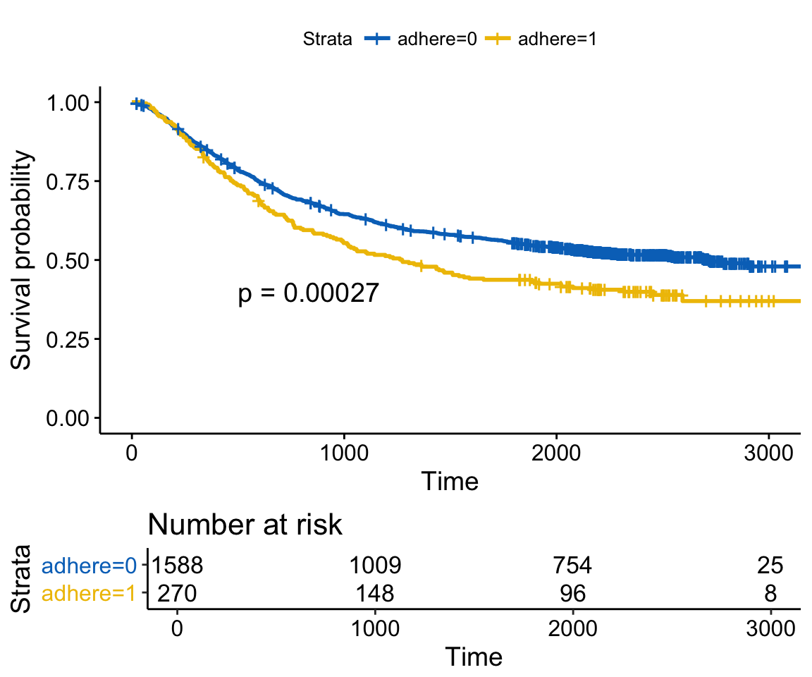
It can be seen that the axes of the survival plot and the risk table are not aligned vertically. To align them, specify the argument align as follow.
ggarrange(ggsurv$plot, ggsurv$table, heights = c(2, 0.7),
          ncol = 1, nrow = 2, align = "v")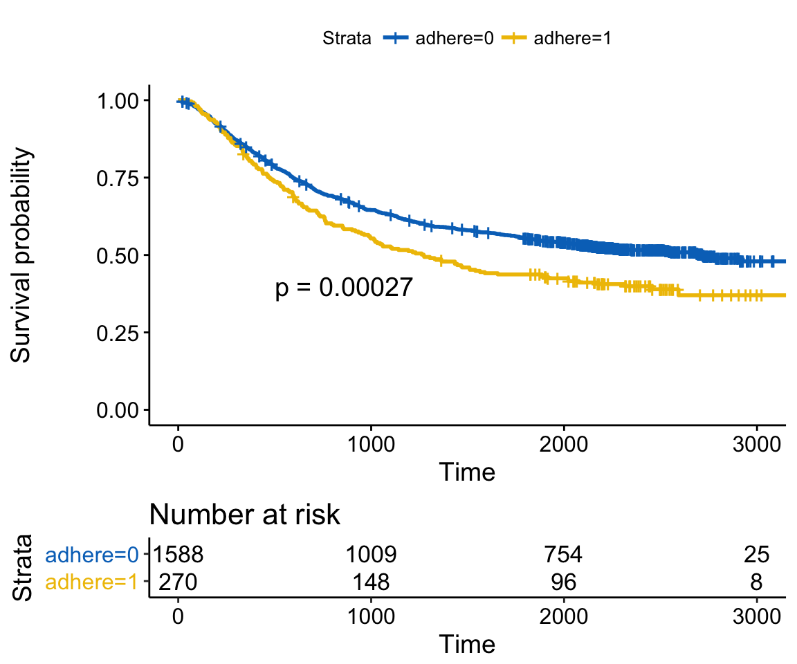
Change column/row span of a plot
Use ggpubr R package
We’ll use nested ggarrange() functions to change column/row span of plots.
For example, using the R code below:
- the scatter plot (sp) will live in the first row and spans over two columns
- the box plot (bxp) and the dot plot (dp) will be first arranged and will live in the second row with two different columns
ggarrange(sp,                                                 # First row with scatter plot
          ggarrange(bxp, dp, ncol = 2, labels = c("B", "C")), # Second row with box and dot plots
          nrow = 2,
          labels = "A"                                        # Labels of the scatter plot
) 
Use cowplot R package
The combination of the functions ggdraw() + draw_plot() + draw_plot_label() [in cowplot] can be used to place graphs at particular locations with a particular size.
ggdraw(). Initialize an empty drawing canvas:
ggdraw()Note that, by default, coordinates run from 0 to 1, and the point (0, 0) is in the lower left corner of the canvas (see the figure below).

draw_plot(). Places a plot somewhere onto the drawing canvas:
draw_plot(plot, x = 0, y = 0, width = 1, height = 1)- plot: the plot to place (ggplot2 or a gtable)
- x, y: The x/y location of the lower left corner of the plot.
- width, height: the width and the height of the plot
draw_plot_label(). Adds a plot label to the upper left corner of a graph. It can handle vectors of labels with associated coordinates.
draw_plot_label(label, x = 0, y = 1, size = 16, ...)- label: a vector of labels to be drawn
- x, y: Vector containing the x and y position of the labels, respectively.
- size: Font size of the label to be drawn
For example, you can combine multiple plots, with particular locations and different sizes, as follow:
library("cowplot")
ggdraw() +
  draw_plot(bxp, x = 0, y = .5, width = .5, height = .5) +
  draw_plot(dp, x = .5, y = .5, width = .5, height = .5) +
  draw_plot(bp, x = 0, y = 0, width = 1, height = 0.5) +
  draw_plot_label(label = c("A", "B", "C"), size = 15,
                  x = c(0, 0.5, 0), y = c(1, 1, 0.5))
Use gridExtra R package
The function arrangeGrop() [in gridExtra] helps to change the row/column span of a plot.
For example, using the R code below:
- the scatter plot (sp) will live in the first row and spans over two columns
- the box plot (bxp) and the dot plot (dp) will live in the second row with two plots in two different columns
library("gridExtra")
grid.arrange(sp,                             # First row with one plot spaning over 2 columns
             arrangeGrob(bxp, dp, ncol = 2), # Second row with 2 plots in 2 different columns
             nrow = 2)                       # Number of rows
It’s also possible to use the argument layout_matrix in the grid.arrange() function, to create a complex layout.
In the R code below layout_matrix is a 2x2 matrix (2 columns and 2 rows). The first row is all 1s, that’s where the first plot lives, spanning the two columns; the second row contains plots 2 and 3 each occupying one column.
grid.arrange(bp,                                    # bar plot spaning two columns
             bxp, sp,                               # box plot and scatter plot
             ncol = 2, nrow = 2,
             layout_matrix = rbind(c(1,1), c(2,3)))
Note that, it’s also possible to annotate the output of the grid.arrange() function using the helper function draw_plot_label() [in cowplot].
To easily annotate the grid.arrange() / arrangeGrob() output (a gtable), you should first transform it to a ggplot using the function as_ggplot() [in ggpubr ]. Next you can annotate it using the function draw_plot_label() [in cowplot].
library("gridExtra")
library("cowplot")
# Arrange plots using arrangeGrob
# returns a gtable (gt)
gt <- arrangeGrob(bp,                               # bar plot spaning two columns
             bxp, sp,                               # box plot and scatter plot
             ncol = 2, nrow = 2,
             layout_matrix = rbind(c(1,1), c(2,3)))
# Add labels to the arranged plots
p <- as_ggplot(gt) +                                # transform to a ggplot
  draw_plot_label(label = c("A", "B", "C"), size = 15,
                  x = c(0, 0, 0.5), y = c(1, 0.5, 0.5)) # Add labels
p
In the above R code, we used arrangeGrob() instead of grid.arrange().
Note that, the main difference between these two functions is that, grid.arrange() draw automatically the output of the arranged plots.
As we want to annotate the arranged plots before drawing it, the function arrangeGrob() is preferred in this case.
Use grid R package
The grid R package can be used to create a complex layout with the help of the function grid.layout(). It provides also the helper function viewport() to define a region or a viewport on the layout. The function print() is used to place plots in a specified region.
The different steps can be summarized as follow :
- Create plots : p1, p2, p3, ….
- Move to a new page on a grid device using the function grid.newpage()
- Create a layout 2X2 - number of columns = 2; number of rows = 2
- Define a grid viewport : a rectangular region on a graphics device
- Print a plot into the viewport
library(grid)
# Move to a new page
grid.newpage()
# Create layout : nrow = 3, ncol = 2
pushViewport(viewport(layout = grid.layout(nrow = 3, ncol = 2)))
# A helper function to define a region on the layout
define_region <- function(row, col){
  viewport(layout.pos.row = row, layout.pos.col = col)
}
# Arrange the plots
print(sp, vp = define_region(row = 1, col = 1:2))   # Span over two columns
print(bxp, vp = define_region(row = 2, col = 1))
print(dp, vp = define_region(row = 2, col = 2))
print(bp + rremove("x.text"), vp = define_region(row = 3, col = 1:2))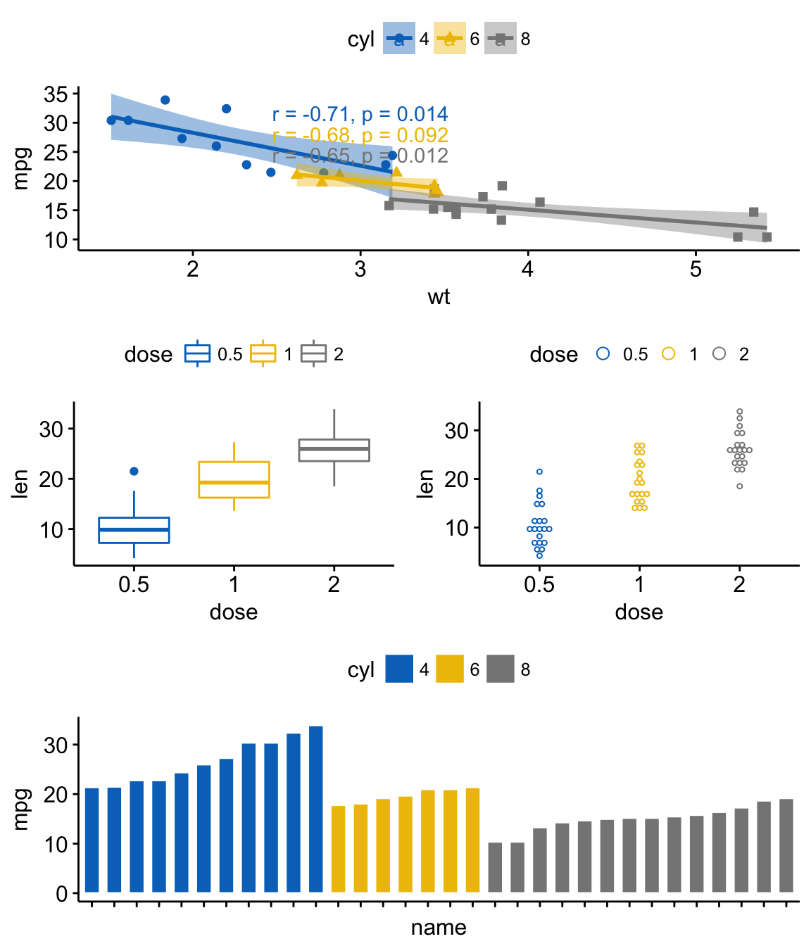
Use common legend for combined ggplots
To place a common unique legend in the margin of the arranged plots, the function ggarrange() [in ggpubr] can be used with the following arguments:
- common.legend = TRUE: place a common legend in a margin
- legend: specify the legend position. Allowed values include one of c(“top”, “bottom”, “left”, “right”)
ggarrange(bxp, dp, labels = c("A", "B"),
          common.legend = TRUE, legend = "bottom")
Scatter plot with marginal density plots
# Scatter plot colored by groups ("Species")
sp <- ggscatter(iris, x = "Sepal.Length", y = "Sepal.Width",
                color = "Species", palette = "jco",
                size = 3, alpha = 0.6)+
  border()
# Marginal density plot of x (top panel) and y (right panel)
xplot <- ggdensity(iris, "Sepal.Length", fill = "Species",
                   palette = "jco")
yplot <- ggdensity(iris, "Sepal.Width", fill = "Species",
                   palette = "jco")+
  rotate()
# Cleaning the plots
yplot <- yplot + clean_theme()
xplot <- xplot + clean_theme()
# Arranging the plot
ggarrange(xplot, NULL, sp, yplot,
          ncol = 2, nrow = 2,  align = "hv",
          widths = c(2, 1), heights = c(1, 2),
          common.legend = TRUE)
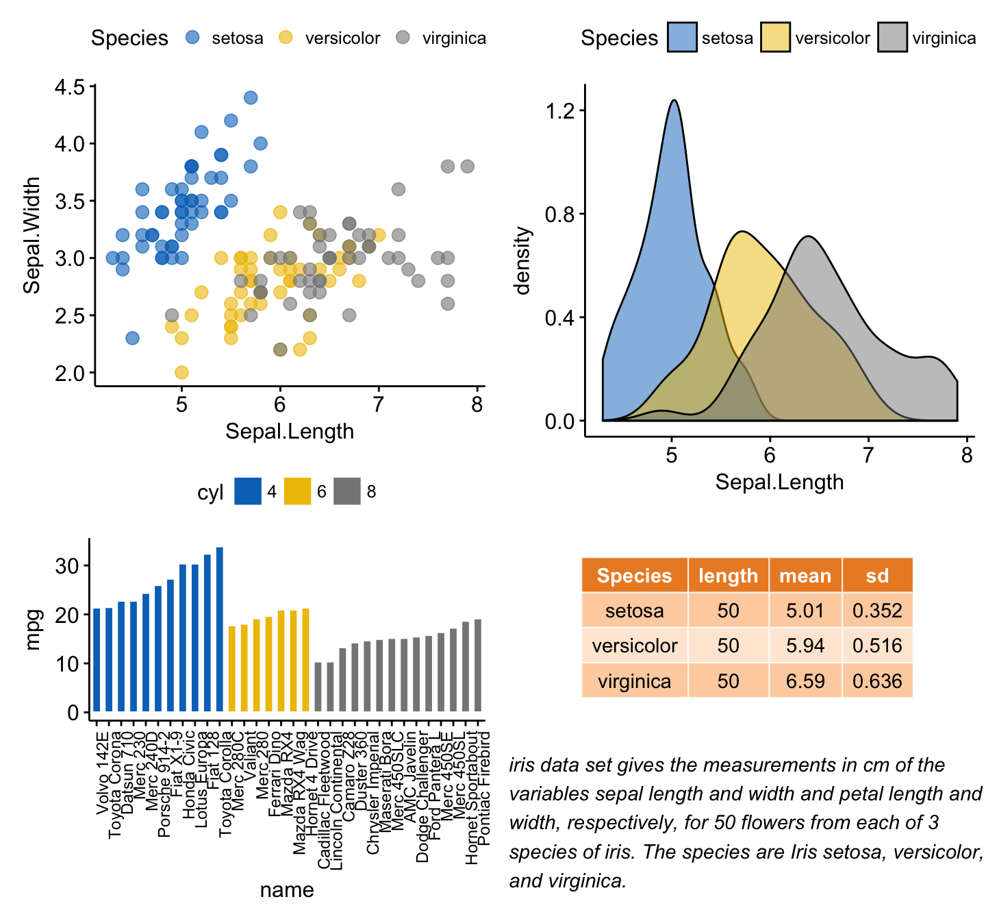
Mix table, text and ggplot2 graphs
In this section, we’ll show how to plot a table and text alongside a chart. The iris data set will be used.
We start by creating the following plots:
- a density plot of the variable “Sepal.Length”. R function: ggdensity() [in ggpubr]
- a plot of the summary table containing the descriptive statistics (mean, sd, … ) of Sepal.Length.
- R function for computing descriptive statistics: desc_statby() [in ggpubr].
- R function to draw a textual table: ggtexttable() [in ggpubr].
- a plot of a text paragraph. R function: ggparagraph() [in ggpubr].
We finish by arranging/combining the three plots using the function ggarrange() [in ggpubr]
# Density plot of "Sepal.Length"
#::::::::::::::::::::::::::::::::::::::
density.p <- ggdensity(iris, x = "Sepal.Length",
                       fill = "Species", palette = "jco")
# Draw the summary table of Sepal.Length
#::::::::::::::::::::::::::::::::::::::
# Compute descriptive statistics by groups
stable <- desc_statby(iris, measure.var = "Sepal.Length",
                      grps = "Species")
stable <- stable[, c("Species", "length", "mean", "sd")]
# Summary table plot, medium orange theme
stable.p <- ggtexttable(stable, rows = NULL,
                        theme = ttheme("mOrange"))
# Draw text
#::::::::::::::::::::::::::::::::::::::
text <- paste("iris data set gives the measurements in cm",
              "of the variables sepal length and width",
              "and petal length and width, respectively,",
              "for 50 flowers from each of 3 species of iris.",
             "The species are Iris setosa, versicolor, and virginica.", sep = " ")
text.p <- ggparagraph(text = text, face = "italic", size = 11, color = "black")
# Arrange the plots on the same page
ggarrange(density.p, stable.p, text.p,
          ncol = 1, nrow = 3,
          heights = c(1, 0.5, 0.3))
Insert a graphical element inside a ggplot
The function annotation_custom() [in ggplot2] can be used for adding tables, plots or other grid-based elements within the plotting area of a ggplot. The simplified format is :
annotation_custom(grob, xmin, xmax, ymin, ymax)- grob: the external graphical element to display
- xmin, xmax : x location in data coordinates (horizontal location)
- ymin, ymax : y location in data coordinates (vertical location)
Place a table within a ggplot
We’ll use the plots - density.p and stable.p - created in the previous section (@ref(mix-table-text-and-ggplot)).
density.p + annotation_custom(ggplotGrob(stable.p),
                              xmin = 5.5, ymin = 0.7,
                              xmax = 8)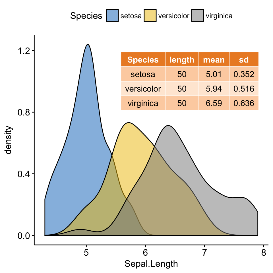
Place a box plot within a ggplot
- Create a scatter plot of y = “Sepal.Width” by x = “Sepal.Length” using the iris data set. R function ggscatter() [ggpubr]
- Create separately the box plot of x and y variables with transparent background. R function: ggboxplot() [ggpubr].
- Transform the box plots into graphical objects called a “grop” in Grid terminology. R function ggplotGrob() [ggplot2].
- Place the box plot grobs inside the scatter plot. R function: annotation_custom() [ggplot2].
As the inset box plot overlaps with some points, a transparent background is used for the box plots.
# Scatter plot colored by groups ("Species")
#::::::::::::::::::::::::::::::::::::::::::::::::::::::::::
sp <- ggscatter(iris, x = "Sepal.Length", y = "Sepal.Width",
                color = "Species", palette = "jco",
                size = 3, alpha = 0.6)
# Create box plots of x/y variables
#::::::::::::::::::::::::::::::::::::::::::::::::::::::::::
# Box plot of the x variable
xbp <- ggboxplot(iris$Sepal.Length, width = 0.3, fill = "lightgray") +
  rotate() +
  theme_transparent()
# Box plot of the y variable
ybp <- ggboxplot(iris$Sepal.Width, width = 0.3, fill = "lightgray") +
  theme_transparent()
# Create the external graphical objects
# called a "grop" in Grid terminology
xbp_grob <- ggplotGrob(xbp)
ybp_grob <- ggplotGrob(ybp)
# Place box plots inside the scatter plot
#::::::::::::::::::::::::::::::::::::::::::::::::::::::::::
xmin <- min(iris$Sepal.Length); xmax <- max(iris$Sepal.Length)
ymin <- min(iris$Sepal.Width); ymax <- max(iris$Sepal.Width)
yoffset <- (1/15)*ymax; xoffset <- (1/15)*xmax
# Insert xbp_grob inside the scatter plot
sp + annotation_custom(grob = xbp_grob, xmin = xmin, xmax = xmax,
                       ymin = ymin-yoffset, ymax = ymin+yoffset) +
  # Insert ybp_grob inside the scatter plot
  annotation_custom(grob = ybp_grob,
                       xmin = xmin-xoffset, xmax = xmin+xoffset,
                       ymin = ymin, ymax = ymax)
Add background image to ggplot2 graphs
Import the background image. Use either the function readJPEG() [in jpeg package] or the function readPNG() [in png package] depending on the format of the background image.
To test the example below, make sure that the png package is installed. You can install it using install.packages(“png”) R command.
# Import the image
img.file <- system.file(file.path("https://www.sthda.com/english/sthda-upload/images/ggpubr", "background-image.png"),
                        package = "ggpubr")
img <- png::readPNG(img.file)
Combine a ggplot with the background image. R function: background_image() [in ggpubr].
library(ggplot2)
library(ggpubr)
ggplot(iris, aes(Species, Sepal.Length))+
  background_image(img)+
  geom_boxplot(aes(fill = Species), color = "white")+
  fill_palette("jco")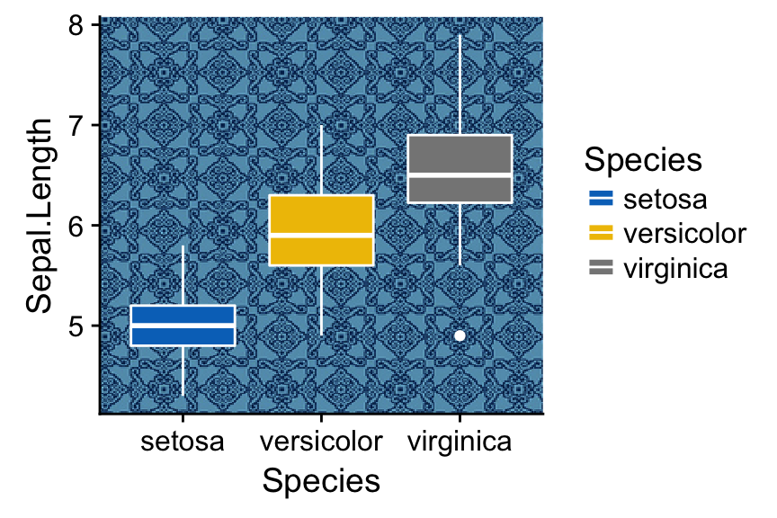
Change box plot fill color transparency by specifying the argument alpha. Value should be in [0, 1], where 0 is full transparency and 1 is no transparency.
library(ggplot2)
library(ggpubr)
ggplot(iris, aes(Species, Sepal.Length))+
  background_image(img)+
  geom_boxplot(aes(fill = Species), color = "white", alpha = 0.5)+
fill_palette("jco")![]()
Another example, overlaying the France map and a ggplot2:
mypngfile <- download.file("https://upload.wikimedia.org/wikipedia/commons/thumb/e/e4/France_Flag_Map.svg/612px-France_Flag_Map.svg.png",
                           destfile = "france.png", mode = 'wb')
img <- png::readPNG('france.png')
ggplot(iris, aes(x = Sepal.Length, y = Sepal.Width)) +
  background_image(img)+
  geom_point(aes(color = Species), alpha = 0.6, size = 5)+
  color_palette("jco")+
  theme(legend.position = "top")
Arrange over multiple pages
If you have a long list of ggplots, say n = 20 plots, you may want to arrange the plots and to place them on multiple pages. With 4 plots per page, you need 5 pages to hold the 20 plots.
The function ggarrange() [in ggpubr] provides a convenient solution to arrange multiple ggplots over multiple pages. After specifying the arguments nrow and ncol, the function ggarrange() computes automatically the number of pages required to hold the list of the plots. It returns a list of arranged ggplots.
For example the following R code,
multi.page <- ggarrange(bxp, dp, bp, sp,
                        nrow = 1, ncol = 2)
returns a list of two pages with two plots per page. You can visualize each page as follow:
multi.page[[1]] # Visualize page 1
multi.page[[2]] # Visualize page 2
You can also export the arranged plots to a pdf file using the function ggexport() [in ggpubr]:
ggexport(multi.page, filename = "multi.page.ggplot2.pdf")PDF file: Multi.page.ggplot2
Note that, it’s also possible to use the function marrangeGrob() [in gridExtra] to create a multi-pages output.
library(gridExtra)
res <- marrangeGrob(list(bxp, dp, bp, sp), nrow = 1, ncol = 2)
# Export to a pdf file
ggexport(res, filename = "multi.page.ggplot2.pdf")
# Visualize interactively
res
Nested layout with ggarrange()
We’ll arrange the plot created in section (@ref(mix-table-text-and-ggplot)) and (@ref(create-some-plots)).
p1 <- ggarrange(sp, bp + font("x.text", size = 9),
                ncol = 1, nrow = 2)
p2 <- ggarrange(density.p, stable.p, text.p,
                ncol = 1, nrow = 3,
                heights = c(1, 0.5, 0.3))
ggarrange(p1, p2, ncol = 2, nrow = 1)
Export plots
R function: ggexport() [in ggpubr].
First, create a list of 4 ggplots corresponding to the variables Sepal.Length, Sepal.Width, Petal.Length and Petal.Width in the iris data set.
plots <- ggboxplot(iris, x = "Species",
                   y = c("Sepal.Length", "Sepal.Width", "Petal.Length", "Petal.Width"),
                   color = "Species", palette = "jco"
                   )
plots[[1]]  # Print the first plot
plots[[2]]  # Print the second plots and so on...
Next, you can export individual plots to a file (pdf, eps or png) (one plot per page). It’s also possible to arrange the plots (2 plot per page) when exporting them.
Export individual plots to a pdf file (one plot per page):
ggexport(plotlist = plots, filename = "test.pdf")Arrange and export. Specify nrow and ncol to display multiple plots on the same page:
ggexport(plotlist = plots, filename = "test.pdf",
         nrow = 2, ncol = 1)
Acknoweledgment
We sincerely thank all developers for their efforts behind the packages that ggpubr depends on, namely:
- Baptiste Auguie (2016). gridExtra: Miscellaneous Functions for “Grid” Graphics. R package version 2.2.1. https://CRAN.R-project.org/package=gridExtra
- Claus O. Wilke (2016). cowplot: Streamlined Plot Theme and Plot Annotations for ‘ggplot2’. R package version 0.7.0. https://CRAN.R-project.org/package=cowplot
- H. Wickham. ggplot2: Elegant Graphics for Data Analysis. Springer-Verlag New York, 2009.