ggplot2.barplot : Easy bar graphs in R software using ggplot2
Introduction
ggplot2.barplot is a function, to plot easily bar graphs using R software and ggplot2 plotting methods. This function is from easyGgplot2 package. An R script is available in the next section to install the package.
The aim of this tutorial is to show you step by step, how to plot and customize a bar chart using ggplot2.barplot function.
At the end of this document you will be able to draw, with few R code, the following plots :
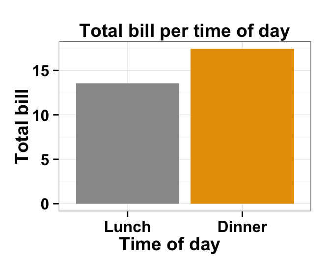

ggplot2.barplot function is described in detail at the end of this document.
Install and load easyGgplot2 package
easyGgplot2 R package can be installed as follow :
install.packages("devtools")
library(devtools)
install_github("easyGgplot2", "kassambara")
Load the package using this R code :
library(easyGgplot2)Data format
The data must be a numeric vector or a data.frame (columns are variables and rows are observations).
restaurant data from easyGgplot2 package will be used in the following example.
#data.frame
head(restaurant)
## sex time total_bill
## 1 Female Lunch 13.53
## 2 Female Dinner 16.81
## 3 Male Lunch 16.24
## 4 Male Dinner 17.42Basic barplot
A subset of restaurant data is used :
df<-restaurant[c(1,4), c("time", "total_bill")]
head(df)
## time total_bill
## 1 Lunch 13.53
## 4 Dinner 17.42# Basic barplot plot of the 2 values of "total_bill" variables
ggplot2.barplot(data=df, xName="time", yName='total_bill')
# Change the width of bars
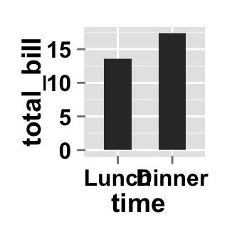
ggplot2.barplot(data=df, xName="time", yName='total_bill',
width=0.5)
# Change the orientation:Horizontal barplot plot
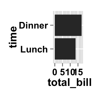
ggplot2.barplot(data=df, xName="time", yName='total_bill',
orientation="horizontal")
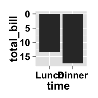
# y Axis reversed
ggplot2.barplot(data=df, xName="time", yName='total_bill',
orientation="yAxisReversed")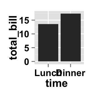
Change the barplot line type and point shape
Different point shapes and line types can be used in the plot. By default, ggplot2 uses solid line type and circle shape.
- The different point shapes in R are described here.
- The available line types are shown here.
ggplot2.barplot(data=df, xName="time", yName='total_bill',
      # Change fill color and line color
      fill="white", color="darkgreen",
      # Change line type and line size
      linetype="dashed", size=1.5)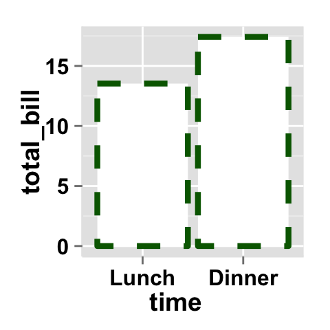
Barplot of counts
In these examples, the height of the bar will represent the count of cases. To get a bar graph of counts, don’t map a variable to yName.
We’ll use the mtcars data :
# Data
head(mtcars)
## mpg cyl disp hp drat wt qsec vs am gear carb
## Mazda RX4 21.0 6 160 110 3.90 2.620 16.46 0 1 4 4
## Mazda RX4 Wag 21.0 6 160 110 3.90 2.875 17.02 0 1 4 4
## Datsun 710 22.8 4 108 93 3.85 2.320 18.61 1 1 4 1
## Hornet 4 Drive 21.4 6 258 110 3.08 3.215 19.44 1 0 3 1
## Hornet Sportabout 18.7 8 360 175 3.15 3.440 17.02 0 0 3 2
## Valiant 18.1 6 225 105 2.76 3.460 20.22 1 0 3 1# Barplot of counts. cyl(for the number of cylenders) is a factor.
# To get a bar graph of counts, don't map a variable to yName.
ggplot2.barplot(data=mtcars, xName="cyl")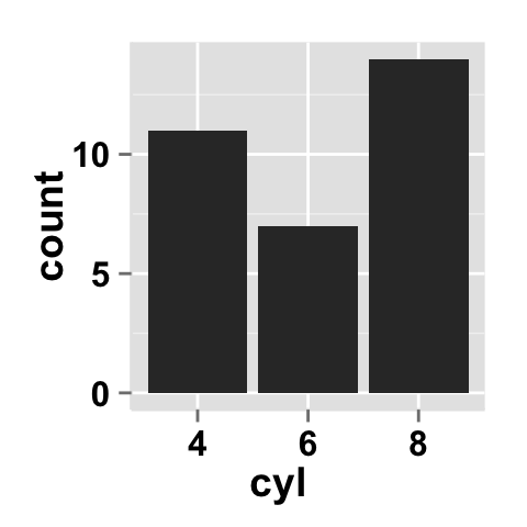
Customize your barplot
Parameters
The arguments that can be used to customize x and y axis are listed below :
| Parameters | Description |
|---|---|
| mainTitle | the title of the plot |
| mainTitleFont | a vector of length 3 indicating respectively the size, the style (“italic”, “bold”, “bold.italic”) and the color of x and y axis titles. Default value is: mainTitleFont=c(14, “bold”, “black”). |
| xShowTitle, yShowTitle | if TRUE, x and y axis titles will be shown. Set the value to FALSE to hide axis labels. Default values are TRUE. |
| xtitle, ytitle | x and y axis labels. Default values are NULL. |
| xtitleFont, ytitleFont | a vector of length 3 indicating respectively the size, the style and the color of x and y axis titles. Possible values for the style:“plain”, “italic”, “bold”, “bold.italic”. Color can be specified as an hexadecimal code (e.g: “#FFCC00”) or by the name (e.g : “red”, “green”). Default values are xtitleFont=c(14,"bold", "black"), ytitleFont=c(14,"bold", "black"). |
| xlim, ylim | limit for the x and y axis. Default values are NULL. |
| xScale, yScale | x and y axis scales. Possible values : c(“none”, “log2”, “log10”). e.g: yScale=“log2”. Default values are NULL. |
| xShowTickLabel, yShowTickLabel | if TRUE, x and y axis tick mark labels will be shown. Default values are TRUE. |
| xTickLabelFont, yTickLabelFont | a vector of length 3 indicating respectively the size, the style and the color of x and y axis tick label fonts. Default value are xTickLabelFont=c(12, "bold", "black"), yTickLabelFont=c(12, "bold", "black"). |
| xtickLabelRotation, ytickLabelRotation | Rotation angle of x and y axis tick labels. Default value are 0. |
| hideAxisTicks | if TRUE, x and y axis ticks are hidden. Default value is FALSE. |
| axisLine | a vector of length 3 indicating respectively the size, the line type and the color of axis lines. Default value is c(0.5, "solid", "#E5E5E5"). |
For more details follow this link : ggplot2.customize.
Main title and axis labels
# Change main title and axis titles
ggplot2.barplot(data=df, xName="time", yName='total_bill',
        mainTitle="Total bill\n per time of day",
        xtitle="Time of day", ytitle="Total bill")
# Customize title styles. Possible values for the font style :
  # 'plain', 'italic', 'bold', 'bold.italic'.
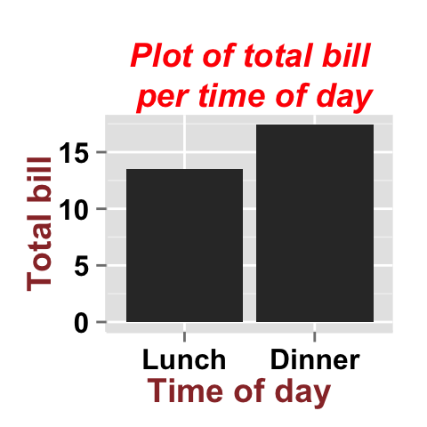
ggplot2.barplot(data=df, xName="time", yName='total_bill',
        mainTitle="Plot of total bill\n per time of day",
        xtitle="Time of day", ytitle="Total bill",
        mainTitleFont=c(14,"bold.italic", "red"),
        xtitleFont=c(14,"bold", "#993333"),
        ytitleFont=c(14,"bold", "#993333"))
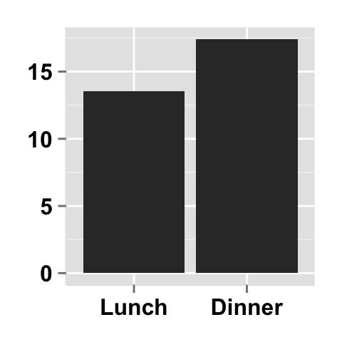
# Hide x an y axis titles
ggplot2.barplot(data=df, xName="time", yName='total_bill',
                xShowTitle=FALSE, yShowTitle=FALSE)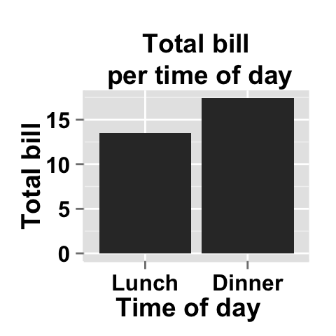
Axis ticks
# Axis ticks labels and orientaion
ggplot2.barplot(data=df, xName="time", yName='total_bill',
        xShowTitle=FALSE, yShowTitle=FALSE,
        xTickLabelFont=c(14,"bold", "#993333"),
        yTickLabelFont=c(14,"bold", "#993333"),
        xtickLabelRotation=45, ytickLabelRotation=45)
#Hide axis tick labels
ggplot2.barplot(data=df, xName="time", yName='total_bill',
        xShowTitle=FALSE, yShowTitle=FALSE,
        xShowTickLabel=FALSE, yShowTickLabel=FALSE)
#Hide axis ticks
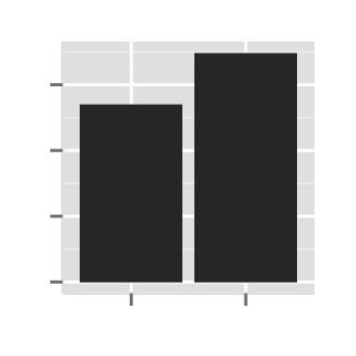
ggplot2.barplot(data=df, xName="time", yName='total_bill',
        xShowTitle=FALSE, yShowTitle=FALSE,
        xShowTickLabel=FALSE, yShowTickLabel=FALSE,
        hideAxisTicks=TRUE)
# AxisLine : a vector of length 3 indicating the size,
  #the line type and the color of axis lines
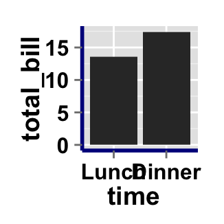
ggplot2.barplot(data=df, xName="time", yName='total_bill',
        axisLine=c(1, "solid", "darkblue"))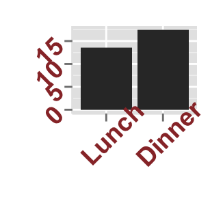

Background and colors
Change barplot background and fill colors
# change background color to "white". Default is "gray"
ggplot2.barplot(data=df, xName="time", yName='total_bill',
          backgroundColor="white")
# Change background color to "lightblue" and grid color to "white"
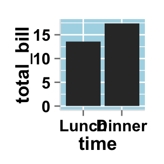
ggplot2.barplot(data=df, xName="time", yName='total_bill',
        backgroundColor="lightblue", gridColor="white")
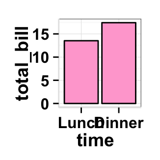
# Change plot fill color
ggplot2.barplot(data=df, xName="time", yName='total_bill',
        backgroundColor="white", fill='#FFAAD4',
        color="black")
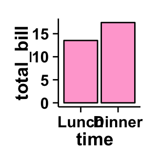
# Remove grid; Remove Top and right border around the plot
ggplot2.barplot(data=df, xName="time", yName='total_bill',
        backgroundColor="white", fill='#FFAAD4', color="black",
        removePanelGrid=TRUE,removePanelBorder=TRUE,
        axisLine=c(0.5, "solid", "black"))
Change barplot color according to the group
Colors can be specified as a hexadecimal RGB triplet, such as "#FFCC00" or by names (e.g : "red" ). You can also use other color scales, such as ones taken from the RColorBrewer package. The different color systems available in R have been described in detail here.
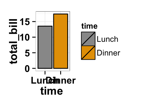
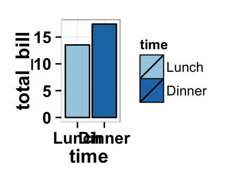
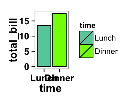
To change barplot color according to the group, you have to specify the name of the data column containing the groups using the argument groupName. Use the argument groupColors, to specify colors by hexadecimal code or by name. In this case, the length of groupColors should be the same as the number of the groups. Use the argument brewerPalette, to specify colors using RColorBrewerpalette.
# Color the barplot by groupName
ggplot2.barplot(data=df, xName="time", yName='total_bill',
                groupName="time")
# Change group colors using hexadecimal colors;
ggplot2.barplot(data=df, xName="time", yName='total_bill',
                groupName="time",
                #background and line colors
                backgroundColor="white", color="black",
                groupColors=c('#999999','#E69F00'))

# Change group colors using brewer palette: "Paired"
ggplot2.barplot(data=df, xName="time", yName='total_bill',
                groupName="time",
                #background and line colors
                backgroundColor="white", color="black",
                brewerPalette="Paired")
# Change group colors using color names
ggplot2.barplot(data=df, xName="time", yName='total_bill',
              groupName="time",
              #background and line colors
              backgroundColor="white", color="black",
              groupColors=c('aquamarine3','chartreuse1'))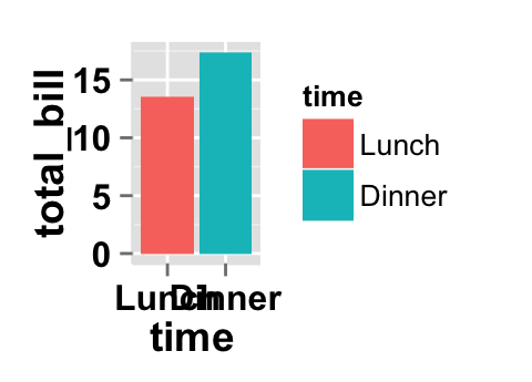
Legend
Legend position
# Change the legend position to "top"
  # (possible values: "left","top", "right", "bottom")
ggplot2.barplot(data=df, xName="time", yName='total_bill',
                groupName="time", legendPosition="top")
# legendPosition can be also a numeric vector c(x, y)
ggplot2.barplot(data=df, xName="time", yName='total_bill',
             groupName="time", legendPosition=c(0.8,0.2))
# Remove plot legend
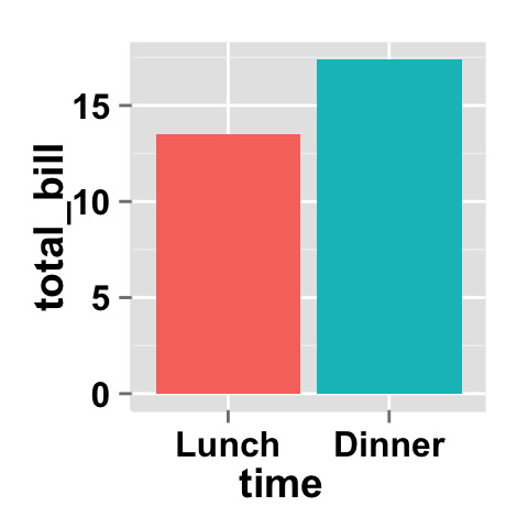
ggplot2.barplot(data=df, xName="time", yName='total_bill',
                groupName="time",showLegend=FALSE)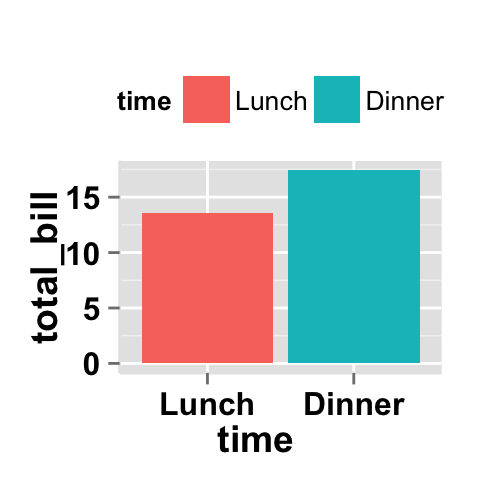
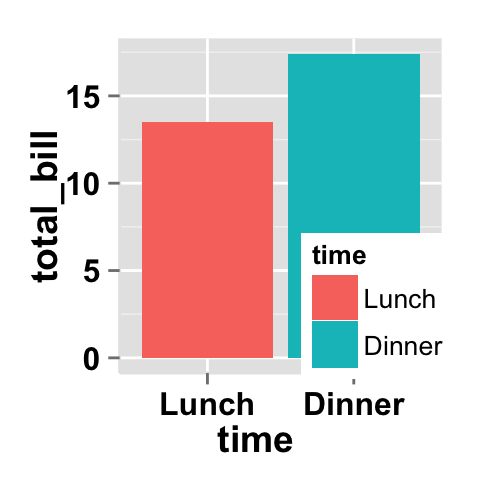
It is also possible to position the legend inside the plotting area. You have to indicate the x, y coordinates of legend box. x and y values must be between 0 and 1. c(0,0) corresponds to “bottom left” and c(1,1) corresponds to “top right” position.
Legend background color, title and text font styles
# Change legend background color, title and text font styles
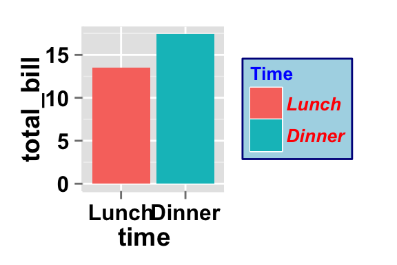
ggplot2.barplot(data=df, xName="time", yName='total_bill',
      groupName="time",
      # legendPosition=c("right", "left","top", "bottom")
      legendPosition="right",
      # legendTitleFont=c(size, style, color)
      legendTitle="Time", legendTitleFont=c(10, "bold", "blue"),
      # legendTextFont=c(size, style, color)
      legendTextFont=c(10, "bold.italic", "red"),
      # legendBackground: c(fill, lineSize, lineType, lineColor)
      legendBackground=c("lightblue", 0.5, "solid", "darkblue" )
      )
Axis scales
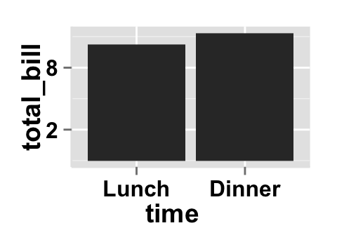
Possible values for y axis scale are “none”, “log2” and log10. Default value is “none”.
# Change y axis limit
ggplot2.barplot(data=df, xName="time", yName='total_bill',
                ylim=c(0,50))

# y Log scale. yScale="log2".
# Possible value="none", "log2" and "log10"
ggplot2.barplot(data=df, xName="time", yName='total_bill',
                yScale="log2")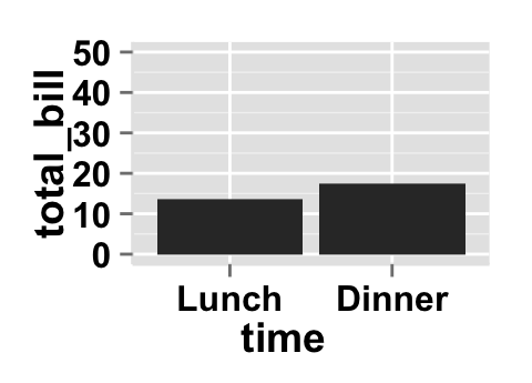
Create a customized plots with few R code
# Customized barplot
ggplot2.barplot(data=df, xName="time", yName='total_bill',
      groupName="time",
      groupColors=c('#999999','#E69F00'), showLegend=FALSE,
      backgroundColor="white", xtitle="Time of day",
      ytitle="Total bill",
      mainTitle="Total bill per \n time of day")
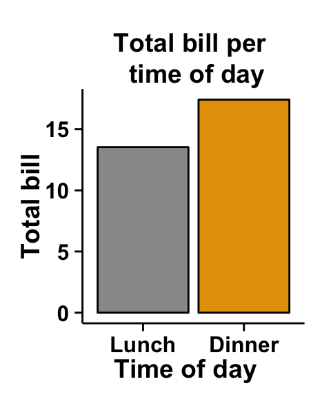
# Remove grid; Remove Top and right border around the plot
ggplot2.barplot(data=df, xName="time", yName='total_bill',
      groupName="time",
      groupColors=c('#999999','#E69F00'), showLegend=FALSE,
      backgroundColor="white", color="black",
      xtitle="Time of day", ytitle="Total bill",
      mainTitle="Total bill per \n time of day",
      removePanelGrid=TRUE,removePanelBorder=TRUE,
      axisLine=c(0.5, "solid", "black"))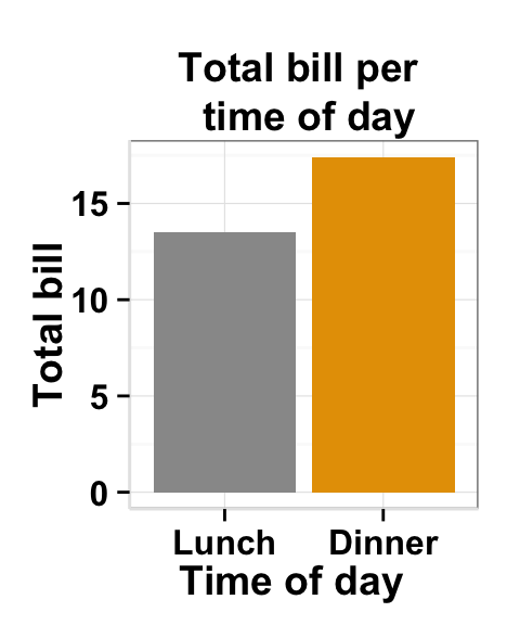
Barplot with multiple groups
This data will be used for the examples below:
df1 <- restaurant
head(df1)
## sex time total_bill
## 1 Female Lunch 13.53
## 2 Female Dinner 16.81
## 3 Male Lunch 16.24
## 4 Male Dinner 17.42# Stacked barplot
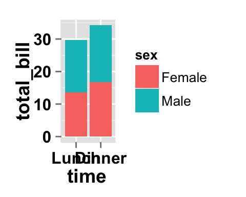
# Plot of variable 'total_bill' according to xName 'time'.
# The plot is colored by the groupName 'sex'
ggplot2.barplot(data=df1, xName='time', yName="total_bill",
groupName='sex')
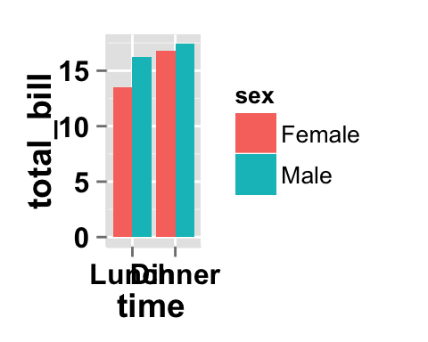
# Use position=position_dodge()
ggplot2.barplot(data=df1, xName='time', yName="total_bill",
groupName='sex', position=position_dodge())
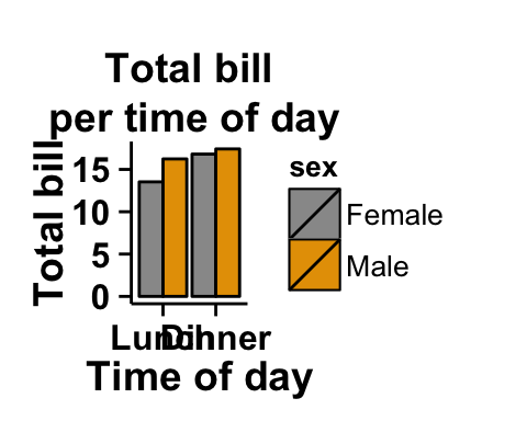
# change colors
ggplot2.barplot(data=df1, xName='time', yName="total_bill",
groupName='sex', groupColors=c('#999999','#E69F00'),
position=position_dodge(),
#background and line colors
backgroundColor="white", color="black",
xtitle="Time of day", ytitle="Total bill",
mainTitle="Total bill\n per time of day",
removePanelGrid=TRUE,removePanelBorder=TRUE,
axisLine=c(0.5, "solid", "black")
) 
In the following examples, diamonds dataset from ggplot2 package is used.
head(diamonds)## carat cut color clarity depth table price x y z
## 1 0.23 Ideal E SI2 61.5 55 326 3.95 3.98 2.43
## 2 0.21 Premium E SI1 59.8 61 326 3.89 3.84 2.31
## 3 0.23 Good E VS1 56.9 65 327 4.05 4.07 2.31
## 4 0.29 Premium I VS2 62.4 58 334 4.20 4.23 2.63
## 5 0.31 Good J SI2 63.3 58 335 4.34 4.35 2.75
## 6 0.24 Very Good J VVS2 62.8 57 336 3.94 3.96 2.48# stacked bar chart; Barplot of the count
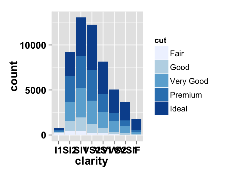
ggplot2.barplot(data=diamonds, xName="clarity",
groupName="cut")
# change the color
ggplot2.barplot(data=diamonds, xName="clarity",
groupName="cut", brewerPalette="Blues")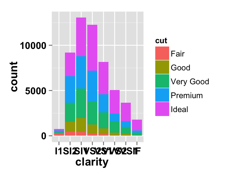
Faceting : split a plot into a matrix of pannels
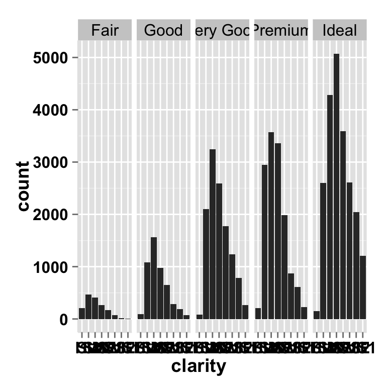
The facet approach splits a plot into a matrix of panels. Each panel shows a different subset of the data.
Facet with one variable
# Facet according to the cut variable
ggplot2.barplot(data=diamonds, xName="clarity",
              faceting=TRUE, facetingVarNames="cut")
# Change the direction.
# possible values are "vertical", "horizontal".
# default is vertical.
ggplot2.barplot(data=diamonds, xName="clarity",
          faceting=TRUE, facetingVarNames="cut",
facetingDirection="horizontal") 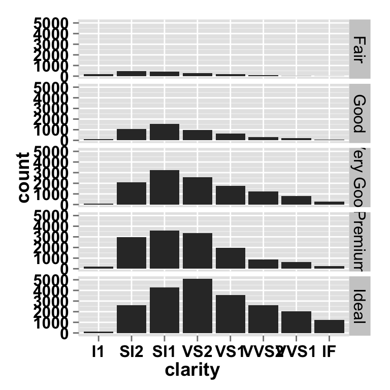
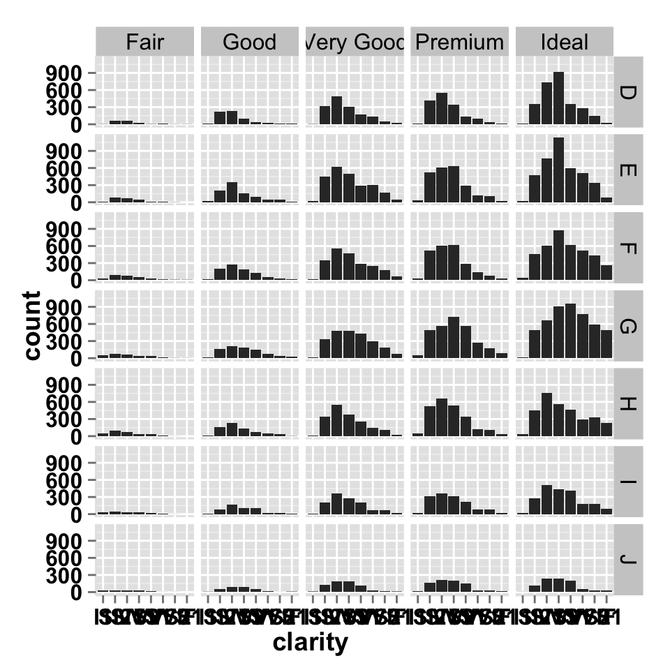
Facet with two variables
# Facet by two variables: cut and color.
# Rows are cut and columns are color
ggplot2.barplot(data=diamonds, xName="clarity",
      faceting=TRUE,
      facetingVarNames=c("cut", "color"))
# Facet by two variables: reverse the order of the 2 variables
# Rows are color and columns are cut
ggplot2.barplot(data=diamonds, xName="clarity",
    faceting=TRUE, facetingVarNames=c( "color", "cut"))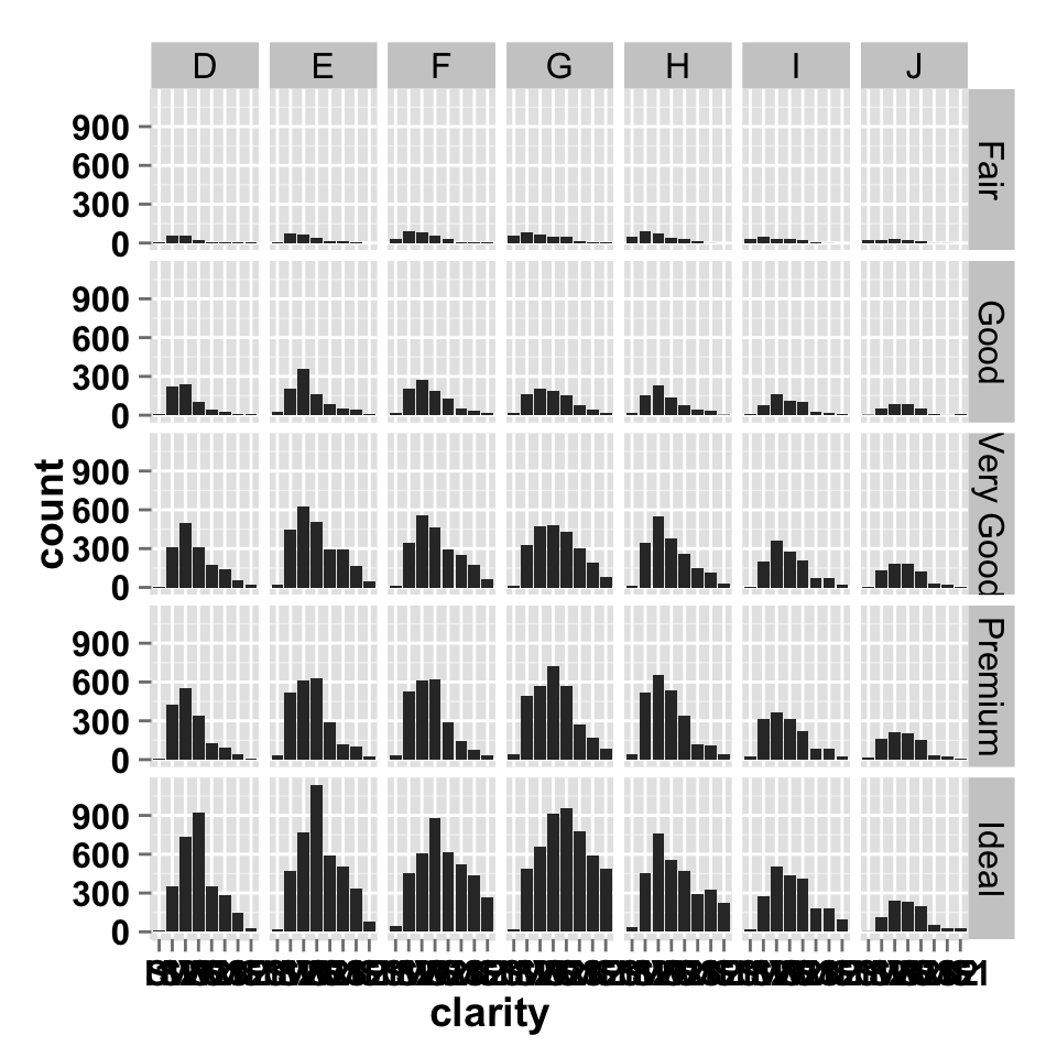
Facet scales
By default, all the panels have the same scale (facetingScales="fixed"). They can be made independent, by setting scales to free, free_x, or free_y.
# Facet with free scales
ggplot2.barplot(data=diamonds, xName="clarity",
      faceting=TRUE, facetingVarNames=c("cut", "color"),
      facetingScales="free")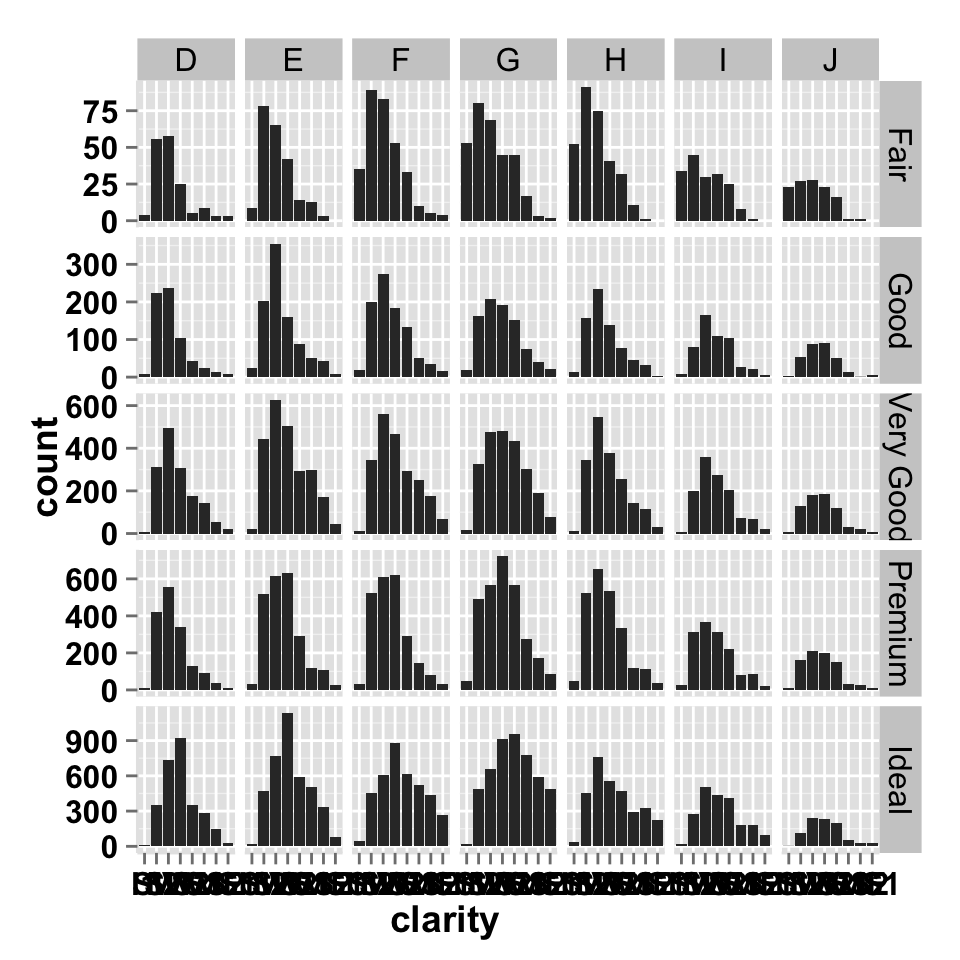
As you can see in the above plot, y axis have different scales in the different panels.
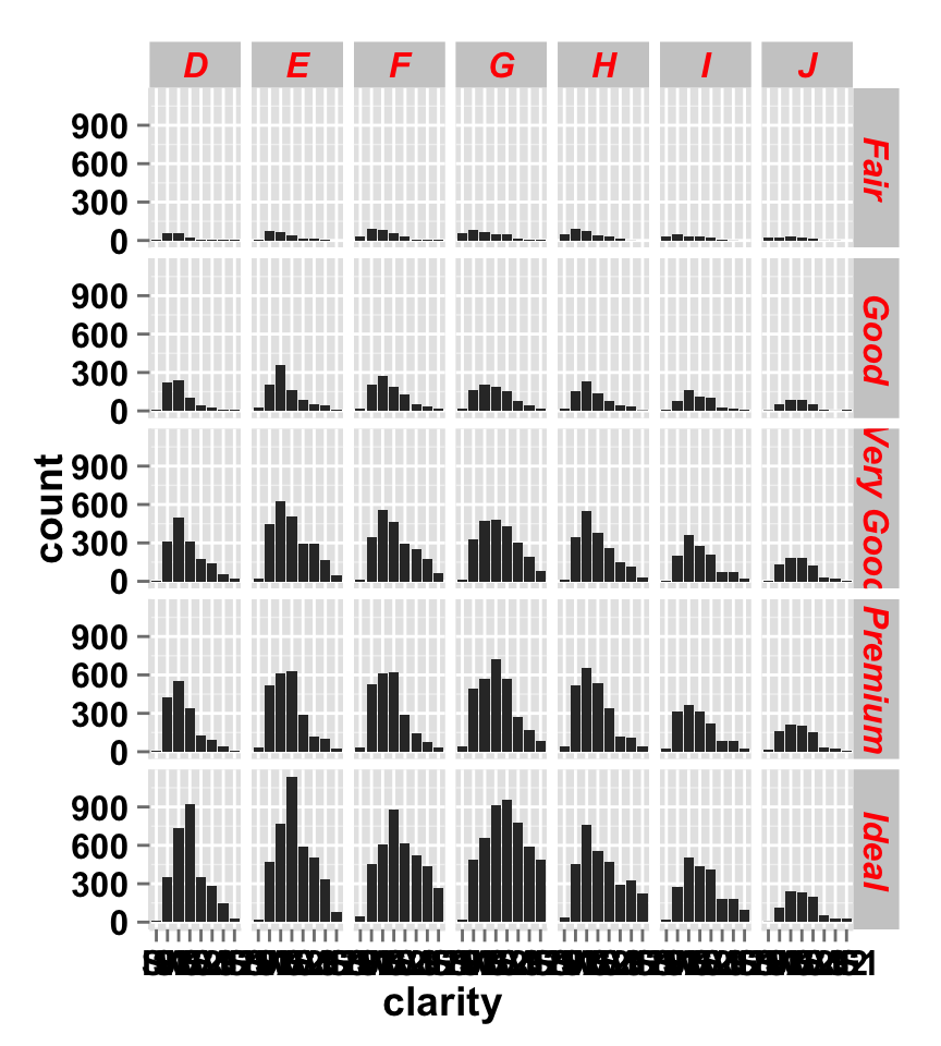
Facet label apperance
# Change facet text font
# Possible values for the font style:'plain', 'italic', 'bold', 'bold.italic'.
ggplot2.barplot(data=diamonds, xName="clarity",
      faceting=TRUE, facetingVarNames=c("cut", "color"),
      facetingFont=c(12, 'bold.italic', "red"))
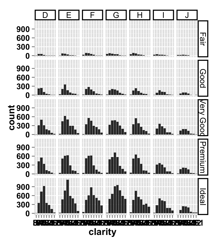
#Change the apperance of the rectangle around facet label
ggplot2.barplot(data=diamonds, xName="clarity",
      faceting=TRUE, facetingVarNames=c("cut", "color"),
      facetingRect=list(background="white", lineType="solid",
                        lineColor="black", lineSize=1.5)
      )
ggplot2.barplot function
Description
Plot easily a barplot using easyGgplot2 R package.
usage
ggplot2.barplot(data, xName=NULL, yName=NULL,
          groupName=NULL,
          groupColors=NULL, brewerPalette=NULL,...)
Arguments
| Arguments | Descriptions |
|---|---|
| data | data.frame or a numeric vector. Columns are variables and rows are observations. |
| xName | The name of column containing x variable (i.e groups). Default value is NULL. |
| yName | The name of column containing y variable. If yName=NULL, data should be a numeric vector. |
| groupName | The name of column containing group variable. This variable is used to color plot according to the group. |
| groupColors | Color of groups. groupColors should have the same length as groups. |
| brewerPalette | This can be also used to indicate group colors. In this case the parameter groupColors should be NULL. e.g: brewerPalette=“Paired”. |
| …. | Other arguments passed on to ggplot2.customize custom function or to geom_bar functions from ggplot2 package. |
The other arguments which can be used are described at this link : ggplot2 customize. They are used to customize the plot (axis, title, background, color, legend, ….) generated using ggplot2 or easyGgplot2 R package.
Examples
library(easyGgplot2)
#data
df <- restaurant[c(1,4), c("time", "total_bill")]
#plot
ggplot2.barplot(data=df, xName="time", yName='total_bill',
        mainTitle="Total bill\n per time of day",
        xtitle="Time of day", ytitle="Total bill")
# Or use this
plot<-ggplot2.barplot(data=df, xName="time", yName='total_bill')
plot<-ggplot2.customize(plot,
            mainTitle="Total bill\n per time of day",
            xtitle="Time of day", ytitle="Total bill")
print(plot)
Easy ggplot2 ebook
Note that an eBook is available on easyGgplot2 package here.
By Alboukadel Kassambara
Copyright 2014 Alboukadel Kassambara. All rights reserved.
Published by STHDA (https://www.sthda.com/english).
September 2014 : First edition.
Licence : This document is under creative commons licence (http://creativecommons.org/licenses/by-nc-sa/3.0/).
Contact : Alboukadel Kassambara alboukadel.kassambara@gmail.com
Infos
This analysis was performed using R (ver. 3.1.0), easyGgplot2 (ver 1.0.0) and ggplot2 (ver 1.0.0).
Show me some love with the like buttons below... Thank you and please don't forget to share and comment below!!
Montrez-moi un peu d'amour avec les like ci-dessous ... Merci et n'oubliez pas, s'il vous plaît, de partager et de commenter ci-dessous!
Recommended for You!
Recommended for you
This section contains the best data science and self-development resources to help you on your path.
Books - Data Science
Our Books
- Practical Guide to Cluster Analysis in R by A. Kassambara (Datanovia)
- Practical Guide To Principal Component Methods in R by A. Kassambara (Datanovia)
- Machine Learning Essentials: Practical Guide in R by A. Kassambara (Datanovia)
- R Graphics Essentials for Great Data Visualization by A. Kassambara (Datanovia)
- GGPlot2 Essentials for Great Data Visualization in R by A. Kassambara (Datanovia)
- Network Analysis and Visualization in R by A. Kassambara (Datanovia)
- Practical Statistics in R for Comparing Groups: Numerical Variables by A. Kassambara (Datanovia)
- Inter-Rater Reliability Essentials: Practical Guide in R by A. Kassambara (Datanovia)
Others
- R for Data Science: Import, Tidy, Transform, Visualize, and Model Data by Hadley Wickham & Garrett Grolemund
- Hands-On Machine Learning with Scikit-Learn, Keras, and TensorFlow: Concepts, Tools, and Techniques to Build Intelligent Systems by Aurelien Géron
- Practical Statistics for Data Scientists: 50 Essential Concepts by Peter Bruce & Andrew Bruce
- Hands-On Programming with R: Write Your Own Functions And Simulations by Garrett Grolemund & Hadley Wickham
- An Introduction to Statistical Learning: with Applications in R by Gareth James et al.
- Deep Learning with R by François Chollet & J.J. Allaire
- Deep Learning with Python by François Chollet
Click to follow us on Facebook :
Comment this article by clicking on "Discussion" button (top-right position of this page)


