


Line Plots - R Base Graphs
Previously, we described the essentials of R programming and provided quick start guides for importing data into R.
Pleleminary tasks
Launch RStudio as described here: Running RStudio and setting up your working directory
Prepare your data as described here: Best practices for preparing your data and save it in an external .txt tab or .csv files
Import your data into R as described here: Fast reading of data from txt|csv files into R: readr package.
R base functions: plot() and lines()
The simplified format of plot() and lines() is as follow.
plot(x, y, type = "l", lty = 1)
lines(x, y, type = "l", lty = 1)- x, y: coordinate vectors of points to join
- type: character indicating the type of plotting. Allowed values are:
- “p” for points
- “l” for lines
- “b” for both points and lines
- “c” for empty points joined by lines
- “o” for overplotted points and lines
- “s” and “S” for stair steps
- “n” does not produce any points or lines
- lty: line types. Line types can either be specified as an integer (0=blank, 1=solid (default), 2=dashed, 3=dotted, 4=dotdash, 5=longdash, 6=twodash) or as one of the character strings “blank”, “solid”, “dashed”, “dotted”, “dotdash”, “longdash”, or “twodash”, where “blank” uses ‘invisible lines’ (i.e., does not draw them).
Create some data
# Create some variables
x <- 1:10
y1 <- x*x
y2  <- 2*y1
We’ll plot a plot with two lines: lines(x, y1) and lines(x, y2).
Note that the function lines() can not produce a plot on its own. However, it can be used to add lines() on an existing graph. This means that, first you have to use the function plot() to create an empty graph and then use the function lines() to add lines.
Basic line plots
# Create a basic stair steps plot
plot(x, y1, type = "S")
# Show both points and line
plot(x, y1, type = "b", pch = 19,
     col = "red", xlab = "x", ylab = "y")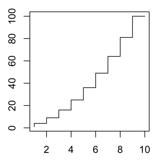

Plots with multiple lines
# Create a first line
plot(x, y1, type = "b", frame = FALSE, pch = 19,
     col = "red", xlab = "x", ylab = "y")
# Add a second line
lines(x, y2, pch = 18, col = "blue", type = "b", lty = 2)
# Add a legend to the plot
legend("topleft", legend=c("Line 1", "Line 2"),
       col=c("red", "blue"), lty = 1:2, cex=0.8)
See also
Infos
This analysis has been performed using R statistical software (ver. 3.2.4).
Show me some love with the like buttons below... Thank you and please don't forget to share and comment below!!
Montrez-moi un peu d'amour avec les like ci-dessous ... Merci et n'oubliez pas, s'il vous plaît, de partager et de commenter ci-dessous!
Recommended for You!


Recommended for you
This section contains the best data science and self-development resources to help you on your path.
Books - Data Science
Our Books
- Practical Guide to Cluster Analysis in R by A. Kassambara (Datanovia)
- Practical Guide To Principal Component Methods in R by A. Kassambara (Datanovia)
- Machine Learning Essentials: Practical Guide in R by A. Kassambara (Datanovia)
- R Graphics Essentials for Great Data Visualization by A. Kassambara (Datanovia)
- GGPlot2 Essentials for Great Data Visualization in R by A. Kassambara (Datanovia)
- Network Analysis and Visualization in R by A. Kassambara (Datanovia)
- Practical Statistics in R for Comparing Groups: Numerical Variables by A. Kassambara (Datanovia)
- Inter-Rater Reliability Essentials: Practical Guide in R by A. Kassambara (Datanovia)
Others
- R for Data Science: Import, Tidy, Transform, Visualize, and Model Data by Hadley Wickham & Garrett Grolemund
- Hands-On Machine Learning with Scikit-Learn, Keras, and TensorFlow: Concepts, Tools, and Techniques to Build Intelligent Systems by Aurelien Géron
- Practical Statistics for Data Scientists: 50 Essential Concepts by Peter Bruce & Andrew Bruce
- Hands-On Programming with R: Write Your Own Functions And Simulations by Garrett Grolemund & Hadley Wickham
- An Introduction to Statistical Learning: with Applications in R by Gareth James et al.
- Deep Learning with R by François Chollet & J.J. Allaire
- Deep Learning with Python by François Chollet
Click to follow us on Facebook :
Comment this article by clicking on "Discussion" button (top-right position of this page)