A complete guide to 3D visualization device system in R - R software and data visualization
- Install the RGL package
- Load the RGL package
- Prepare the data
- Start and close RGL device
- 3D scatter plot
- rgl_init(): A custom function to initialize RGL device
- Add a bounding box decoration
- Add axis lines and labels
- Set the aspect ratios of the x, y and z axes
- Change the color of points by groups
- Change the shape of points
- Add an ellipse of concentration
- Regression plane
- Create a movie of RGL scene
- Export images as png or pdf
- Export the plot into an interactive HTML file
- Select a rectangle in an RGL scene
- Identify points in a plot
- R3D Interface
- RGL functions
- Infos
This R tutorial describes, step by step, how to build a 3D graphic using R software and the rgl package. You’ll learn also how to create a movie of your 3D scene in R.
RGL is a 3D graphics package that produces a real-time interactive 3D plot. It allows to interactively rotate, zoom the graphics and select regions.
The rgl package includes also a generic 3D interface named R3D. R3D is a collection of generic 3D objects and functions which are described at the end of this article.
Install the RGL package
install.packages("rgl")Note that, on Linux operating system, the rgl package can be installed as follow:
sudo apt-get install r-cran-rgl
Load the RGL package
library("rgl")Prepare the data
We’ll use the iris data set in the following examples:
data(iris)
head(iris)
Sepal.Length Sepal.Width Petal.Length Petal.Width Species
1 5.1 3.5 1.4 0.2 setosa
2 4.9 3.0 1.4 0.2 setosa
3 4.7 3.2 1.3 0.2 setosa
4 4.6 3.1 1.5 0.2 setosa
5 5.0 3.6 1.4 0.2 setosa
6 5.4 3.9 1.7 0.4 setosax <- sep.l <- iris$Sepal.Length
y <- pet.l <- iris$Petal.Length
z <- sep.w <- iris$Sepal.Widthiris data set gives the measurements of the variables sepal length and width, petal length and width, respectively, for 50 flowers from each of 3 species of iris. The species are Iris setosa, versicolor, and virginica.
Start and close RGL device
To make a 3D plot with RGL, you should first start the RGL device in R.
The functions below are used to manage the RGL device:
- rgl.open(): Opens a new device
- rgl.close(): Closes the current device
- rgl.clear(): Clears the current device
- rgl.cur(): Returns the active device ID
- rgl.quit(): Shutdowns the RGL device system
In the first sections of this tutorial, I’ll open a new RGL device for each plot.
Note that, you don’t need to do the same thing.
You can just use the function rgl.open() the first time –> then make your first 3D plot –> then use rgl.clear() to clear the scene –> and make a new plot again.3D scatter plot
Basic graph
The function rgl.points() is used to draw a 3D scatter plot:
rgl.open() # Open a new RGL device
rgl.points(x, y, z, color ="lightgray") # Scatter plot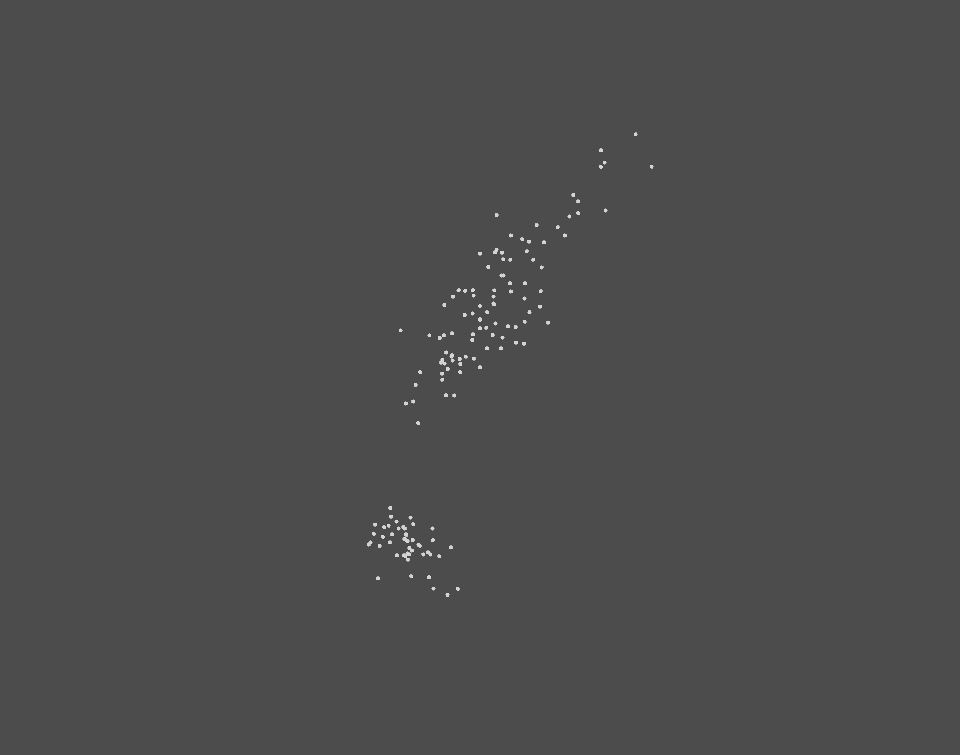
- x, y, z : Numeric vector specifying the coordinates of points to be drawn. The arguments y and z are optional when:
- x is a matrix or a data frame containing at least 3 columns which will be used as the x, y and z coordinates. Ex: rgl.points(iris)
- x is a formula of form zvar ~ xvar + yvar (see ?xyz.coords). Ex: rgl.points( z ~ x + y).
- …: Material properties. See ?rgl.material for details.
Change the background and point colors
- The function rgl.bg(color) can be used to setup the background environment of the scene
- The argument color is used in the function rgl.points() to change point colors
Note that, it’s also possible to change the size of points using the argument size
rgl.open()# Open a new RGL device
rgl.bg(color = "white") # Setup the background color
rgl.points(x, y, z, color = "blue", size = 5) # Scatter plot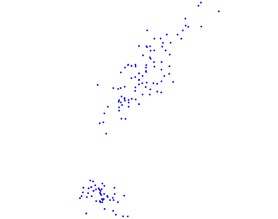
Note that, the equivalent of the functions above for the 3d interface is:
- open3d(): Open a new 3D device
- bg3d(color): Set up the background environment of the scene
- points3d(x, y, Z, …): plot points of coordinates x, y, z
Change the shape of points
It’s possible to draw spheres using the functions rgl.spheres() or spheres3d():
spheres3d(x, y = NULL, z = NULL, radius = 1, ...)
rgl.spheres(x, y = NULL, z = NULL, r, ...)
rgl.spheres() draws spheres with center (x, y, z) and radius r.
- x, y, z : Numeric vector specifying the coordinates for the center of each sphere. The arguments y and z are optional when:
- x is a matrix or a data frame containing at least 3 columns which will be used as the x, y and z coordinates. Ex: rgl.spheres(iris, r = 0.2)
- x is a formula of form zvar ~ xvar + yvar (see ?xyz.coords). Ex: rgl.spheres( z ~ x + y, r = 0.2).
- radius: a vector or single value indicating the radius of spheres
- …: Material properties. See ?rgl.material for details.
rgl.open()# Open a new RGL device
rgl.bg(color = "white") # Setup the background color
rgl.spheres(x, y, z, r = 0.2, color = "grey") 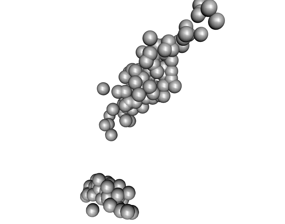
Note that, an rgl plot can be manually rotated by holding down on the mouse or touchpad. It can be also zoomed using the scroll wheel on a mouse or pressing ctrl + using the touchpad on a PC or two fingers (up or down) on a mac.
rgl_init(): A custom function to initialize RGL device
The function rgl_init() will create a new RGL device if requested or if there is no opened device:
#' @param new.device a logical value. If TRUE, creates a new device
#' @param bg the background color of the device
#' @param width the width of the device
rgl_init <- function(new.device = FALSE, bg = "white", width = 640) {
  if( new.device | rgl.cur() == 0 ) {
    rgl.open()
    par3d(windowRect = 50 + c( 0, 0, width, width ) )
    rgl.bg(color = bg )
  }
  rgl.clear(type = c("shapes", "bboxdeco"))
  rgl.viewpoint(theta = 15, phi = 20, zoom = 0.7)
}
Description of the used RGL functions:
- rgl.open(): open a new device
- rgl.cur(): returns active device ID
- par3d(windowRect): set the window size
- rgl.viewpoint(theta, phi, fov, zoom): set up viewpoint. The arguments theta and phi are polar coordinates.
- theta and phi are the polar coordinates. Default values are 0 and 15, respectively
- fov is the field-of-view angle in degrees. Default value is 60
- zoom is the zoom factor. Default value is 1
- rgl.bg(color): define the background color of the device
- rgl.clear(type): Clears the scene from the specified stack (“shapes”, “lights”, “bboxdeco”, “background”)
In the R code above, I used the function rgl.viewpoint() to set automatically the viewpoint orientation and the zoom. As you already know, the RGL device is interactive and you can adjust the viewpoint and zoom the plot using your mouse.
Add a bounding box decoration
The function rgl.bbox() is used:
rgl_init()
rgl.spheres(x, y, z, r = 0.2, color = "yellow")  # Scatter plot
rgl.bbox(color = "#333377") # Add bounding box decoration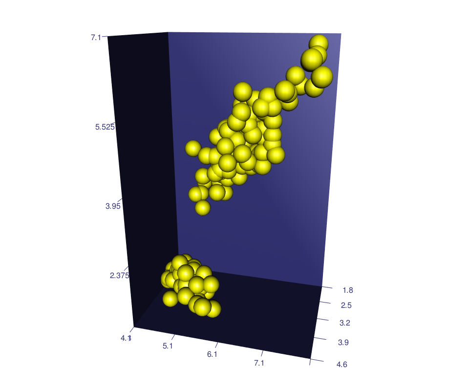
A simplified format of the function rgl.bbox() is:
rgl.bbox(xlen=5, ylen=5, zlen=5, marklen=15.9, ...)- xlen, ylen, zlen: values specifying the number of tickmarks on x, y and Z axes, respectively
- marklen: value specifying the length of the tickmarks
- …: other rgl material properties (see ?rgl.material) including:
- color: a vector of colors. The first color is used for the background color of the bounding box. The second color is used for the tick mark labels.
- emission, specular, shininess: properties for lighting calculation
- alpha: value specifying the color transparency. The value should be between 0.0 (fully transparent) and 1.0 (opaque)
rgl_init()
rgl.spheres(x, y, z, r = 0.2, color = "yellow")
# Add bounding box decoration
rgl.bbox(color=c("#333377","black"), emission="#333377",
specular="#3333FF", shininess=5, alpha=0.8 ) 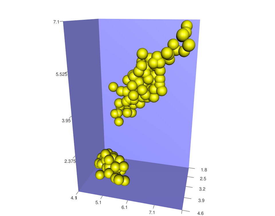
Add axis lines and labels
- The function rgl.lines(x, y = NULL, z = NULL, …) can be used to add axis lines.
- The function rgl.texts(x, y = NULL, z = NULL, text) is used to add axis labels
For the function rgl.lines(), the arguments x, y, and z are numeric vectors of length 2 (i.e, : x = c(x1,x2), y = c(y1, y2), z = c(z1, z2) ).
- The values x1, y1 and y3 are the 3D coordinates of the line starting point.
- The values x2, y2 and y3 corresponds to the 3D coordinates of the line ending point.
Note also that, the argument x can be a matrix or a data frame containing, at least, 3 columns corresponding to the x, y and z coordinates, respectively. In this case, the argument y and z can be omitted.
To draw an axis, you should specify the range (minimum and the maximum) of the axis to the function rgl.lines():
# Make a scatter plot
rgl_init()
rgl.spheres(x, y, z, r = 0.2, color = "yellow")
# Add x, y, and z Axes
rgl.lines(c(min(x), max(x)), c(0, 0), c(0, 0), color = "black")
rgl.lines(c(0, 0), c(min(y),max(y)), c(0, 0), color = "red")
rgl.lines(c(0, 0), c(0, 0), c(min(z),max(z)), color = "green")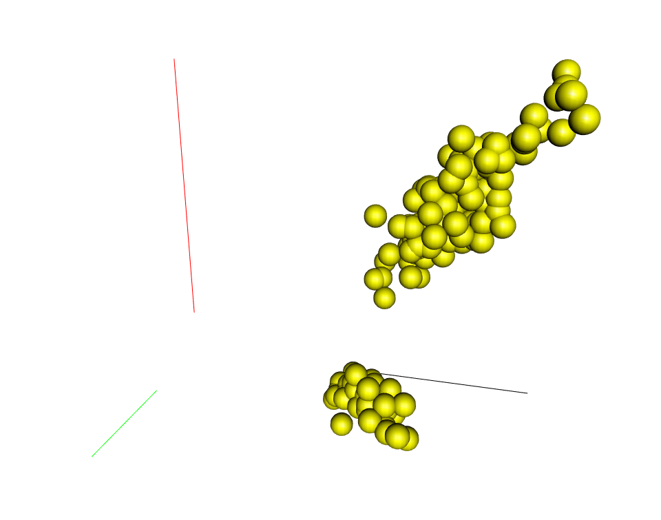
As you can see, the axes are drawn but the problem is that they don’t cross at the point c(0, 0, 0)
There are two solutions to handle this situation:
- Scale the data to make things easy. Transform the x, y and z variables so that their min = 0 and their max = 1
- Use c(-max, +max) as the ranges of the axes
Scale the data
x1 <- (x - min(x))/(max(x) - min(x))
y1 <- (y - min(y))/(max(y) - min(y))
z1 <- (z - min(z))/(max(z) - min(z))
# Make a scatter plot
rgl_init()
rgl.spheres(x1, y1, z1, r = 0.02, color = "yellow")
# Add x, y, and z Axes
rgl.lines(c(0, 1), c(0, 0), c(0, 0), color = "black")
rgl.lines(c(0, 0), c(0,1), c(0, 0), color = "red")
rgl.lines(c(0, 0), c(0, 0), c(0,1), color = "green")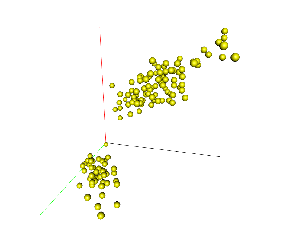
Use c(-max, max)
Let’s define a helper function to calculate the axis limits:
lim <- function(x){c(-max(abs(x)), max(abs(x))) * 1.1}# Make a scatter plot
rgl_init()
rgl.spheres(x, y, z, r = 0.2, color = "yellow")
# Add x, y, and z Axes
rgl.lines(lim(x), c(0, 0), c(0, 0), color = "black")
rgl.lines(c(0, 0), lim(y), c(0, 0), color = "red")
rgl.lines(c(0, 0), c(0, 0), lim(z), color = "green")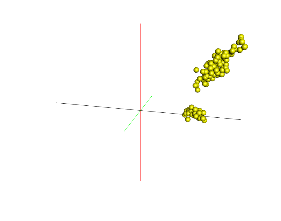
rgl_add_axes(): A custom function to add x, y and z axes
# x, y, z : numeric vectors corresponding to
#  the coordinates of points
# axis.col : axis colors
# xlab, ylab, zlab: axis labels
# show.plane : add axis planes
# show.bbox : add the bounding box decoration
# bbox.col: the bounding box colors. The first color is the
# the background color; the second color is the color of tick marks
rgl_add_axes <- function(x, y, z, axis.col = "grey",
                xlab = "", ylab="", zlab="", show.plane = TRUE,
                show.bbox = FALSE, bbox.col = c("#333377","black"))
  {

  lim <- function(x){c(-max(abs(x)), max(abs(x))) * 1.1}
  # Add axes
  xlim <- lim(x); ylim <- lim(y); zlim <- lim(z)
  rgl.lines(xlim, c(0, 0), c(0, 0), color = axis.col)
  rgl.lines(c(0, 0), ylim, c(0, 0), color = axis.col)
  rgl.lines(c(0, 0), c(0, 0), zlim, color = axis.col)

   # Add a point at the end of each axes to specify the direction
   axes <- rbind(c(xlim[2], 0, 0), c(0, ylim[2], 0),
                 c(0, 0, zlim[2]))
   rgl.points(axes, color = axis.col, size = 3)

  # Add axis labels
  rgl.texts(axes, text = c(xlab, ylab, zlab), color = axis.col,
             adj = c(0.5, -0.8), size = 2)

  # Add plane
  if(show.plane)
    xlim <- xlim/1.1; zlim <- zlim /1.1
    rgl.quads( x = rep(xlim, each = 2), y = c(0, 0, 0, 0),
             z = c(zlim[1], zlim[2], zlim[2], zlim[1]))

  # Add bounding box decoration
  if(show.bbox){
    rgl.bbox(color=c(bbox.col[1],bbox.col[2]), alpha = 0.5,
          emission=bbox.col[1], specular=bbox.col[1], shininess=5,
          xlen = 3, ylen = 3, zlen = 3)
  }
}- The function rgl.texts(x, y, z, text ) is used to add texts to an RGL plot.
- rgl.quads(x, y, z) is used to add planes. x, y and z are numeric vectors of length four specifying the coordinates of the four nodes of the quad.
rgl_init()
rgl.spheres(x, y, z, r = 0.2, color = "yellow")
rgl_add_axes(x, y, z)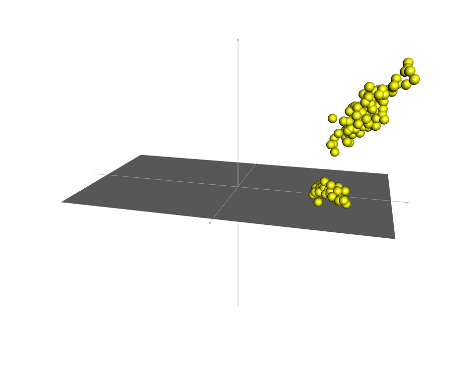
Show scales: tick marks
The function axis3d() can be used as follow:
rgl_init()
rgl.spheres(x, y, z, r = 0.2, color = "yellow")
rgl_add_axes(x, y, z)
# Show tick marks
axis3d('x', pos=c( NA, 0, 0 ), col = "darkgrey")
axis3d('y', pos=c( 0, NA, 0 ), col = "darkgrey")
axis3d('z', pos=c( 0, 0, NA ), col = "darkgrey")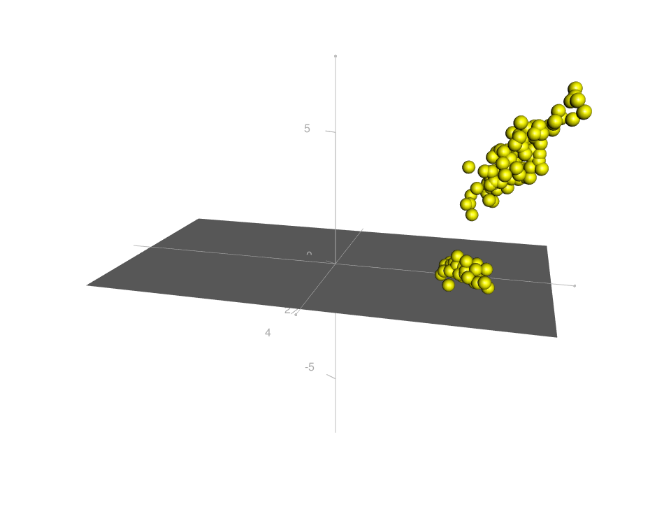
It’s easier to just add a bounding box decoration:
rgl_init()
rgl.spheres(x, y, z, r = 0.2, color = "yellow")
rgl_add_axes(x, y, z, show.bbox = TRUE)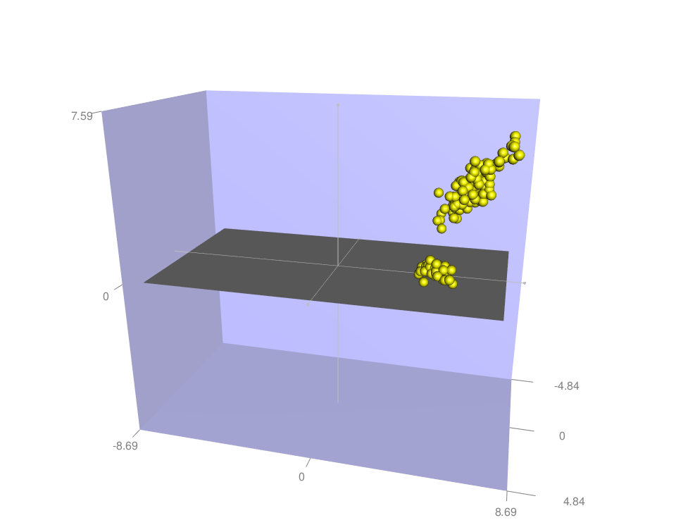
Set the aspect ratios of the x, y and z axes
In the plot above, the bounding box is displayed as rectangle. All the coordinates are displayed at the same scale (iso-metric).
The function aspect3d(x, y = NULL, z = NULL) can be used to set the apparent ratios of the x, y and z axes for the current plot.
x, y and z are the ratio for x, y and z axes, respectively. x can be a vector of length 3, specifying the ratio for the 3 axes.
If the ratios are (1, 1, 1), the bounding box will be displayed as a cube.
rgl_init()
rgl.spheres(x, y, z, r = 0.2, color = "yellow")
rgl_add_axes(x, y, z, show.bbox = TRUE)
aspect3d(1,1,1)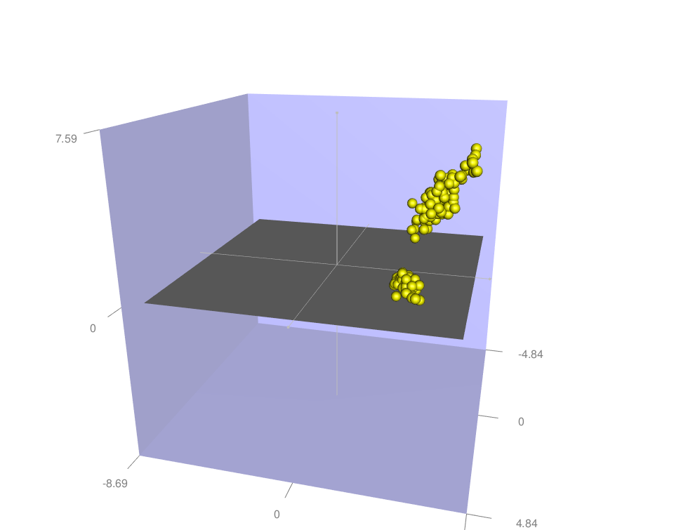
Note that, the default display corresponds to the aspect “iso”: aspect3d(“iso”).
The values of the ratios can be set larger or smaller to zoom on a given axis:
rgl_init()
rgl.spheres(x, y, z, r = 0.2, color = "yellow")
rgl_add_axes(x, y, z, show.bbox = TRUE)
aspect3d(2,1,1) # zoom on x axis
Change the color of points by groups
A helper function can be used to select automatically a color for each group:
#' Get colors for the different levels of
#' a factor variable
#'
#' @param groups a factor variable containing the groups
#'  of observations
#' @param colors a vector containing the names of
#   the default colors to be used
get_colors <- function(groups, group.col = palette()){
  groups <- as.factor(groups)
  ngrps <- length(levels(groups))
  if(ngrps > length(group.col))
    group.col <- rep(group.col, ngrps)
  color <- group.col[as.numeric(groups)]
  names(color) <- as.vector(groups)
  return(color)
}
Change colors by groups :
rgl_init()
rgl.spheres(x, y, z, r = 0.2,
          color = get_colors(iris$Species))
rgl_add_axes(x, y, z, show.bbox = TRUE)
aspect3d(1,1,1)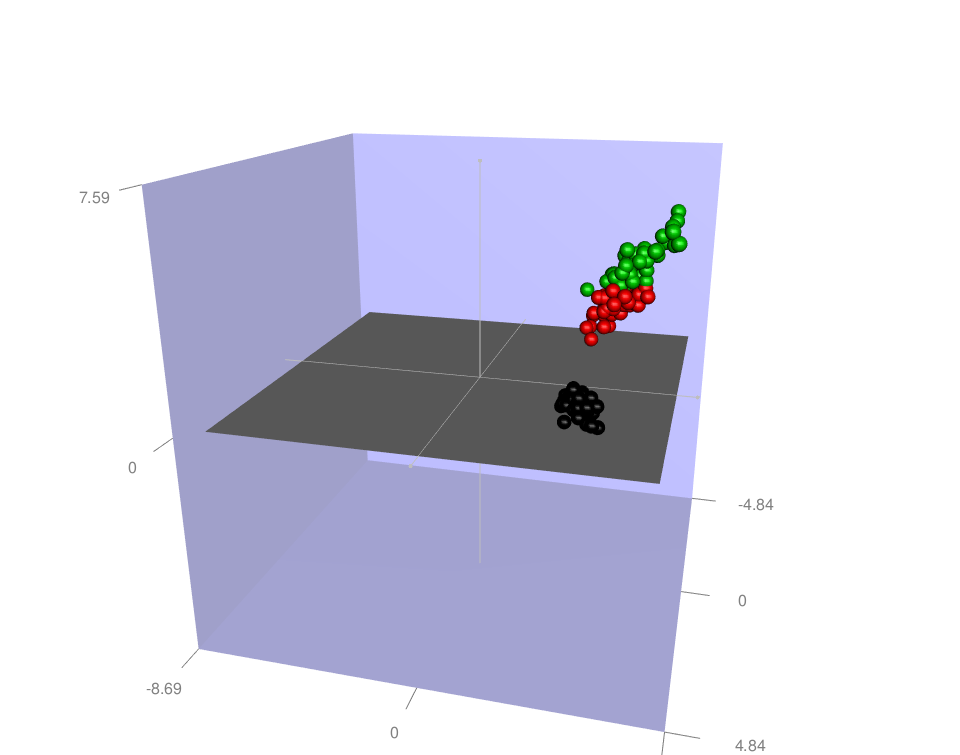
Use custom colors:
cols <- get_colors(iris$Species, c("#999999", "#E69F00", "#56B4E9"))
rgl_init()
rgl.spheres(x, y, z, r = 0.2, color = cols)
rgl_add_axes(x, y, z, show.bbox = TRUE)
aspect3d(1,1,1)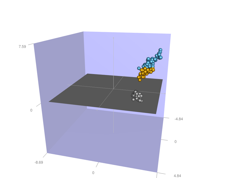
It’s also possible to use color palettes from the RColorBrewer package:
library("RColorBrewer")
cols <- get_colors(iris$Species, brewer.pal(n=3, name="Dark2") )
rgl_init()
rgl.spheres(x, y, z, r = 0.2, color = cols)
rgl_add_axes(x, y, z, show.bbox = TRUE)
aspect3d(1,1,1)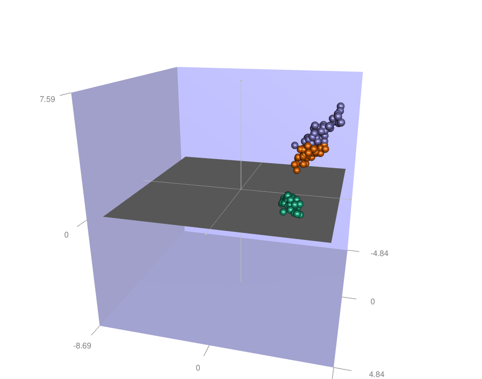
Read more about colors in R: colors in R
Change the shape of points
6 mesh objects are available in RGL package and can be used as point shapes:
- cube3d()
- tetrahedron3d()
- octahedron3d()
- icosahedron3d()
- dodecahedron3d()
- cuboctahedron3d()
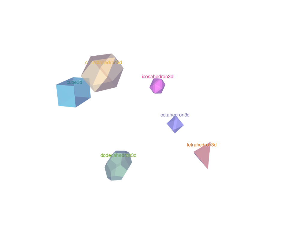
To make a plot using the objects above, the function shapelist3d() can be used as follow:
shapelist3d(shapes, x, y, z)- shapes: a single shape3d (ex: shapes = cube3d()) object or a list of them (ex: shapes = list(cube3d(), icosahedron3d()))
- x, y, z: the coordinates of the points to be plotted
rgl_init()
shapelist3d(tetrahedron3d(), x, y, z, size =  0.15,
            color = get_colors(iris$Species))
rgl_add_axes(x, y, z, show.bbox = TRUE)
aspect3d(1,1,1)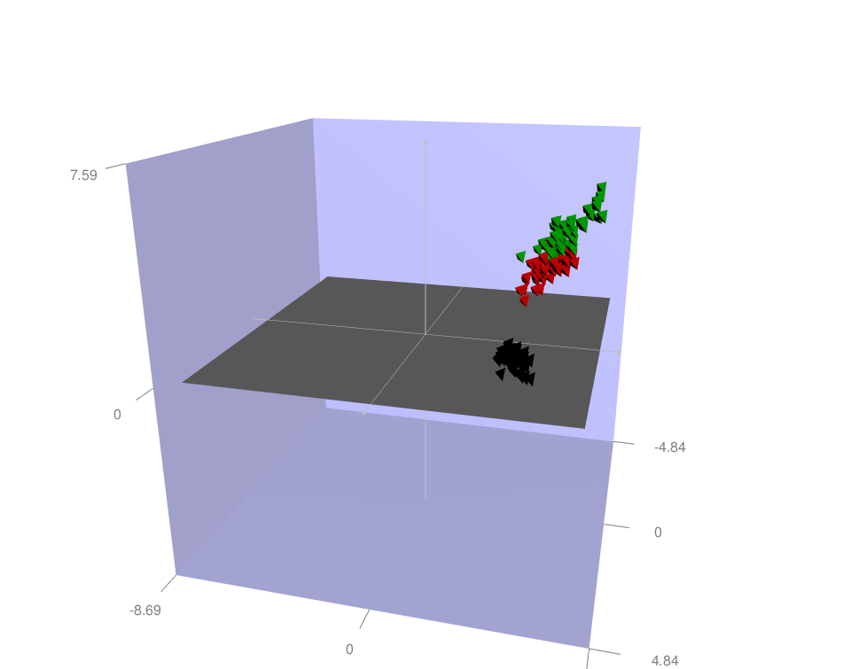
Add an ellipse of concentration
The function ellipse3d() is used to estimate the ellipse of concentration. A simplified format is:
ellipse3d(x, scale = c(1,1,1), centre = c(0,0,0),
level = 0.95, ...)- x: the correlation or covariance matrix between x, y and z
- scale: If x is a correlation matrix, then the standard deviations of each parameter can be given in the scale parameter. This defaults to c(1, 1, 1), so no rescaling will be done.
- centre: The center of the ellipse will be at this position.
- level: The confidence level of a confidence region. This is used to control the size of the ellipsoid.
The function ellipse3d() returns an object of class mesh3d which can be drawn using the function shade3d() and/or wired3d()
- Draw the ellipse using the function shade3d():
rgl_init()
rgl.spheres(x, y, z, r = 0.2, color = "#D95F02")
rgl_add_axes(x, y, z, show.bbox = TRUE)
# Compute and draw the ellipse of concentration
ellips <- ellipse3d(cov(cbind(x,y,z)),
            centre=c(mean(x), mean(y), mean(z)), level = 0.95)
shade3d(ellips, col = "#D95F02", alpha = 0.1, lit = FALSE)
aspect3d(1,1,1)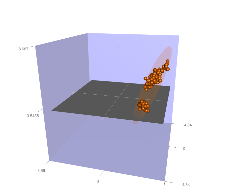
- Draw the ellipse using the function wired3d():
rgl_init()
rgl.spheres(x, y, z, r = 0.2, color = "#D95F02")
rgl_add_axes(x, y, z, show.bbox = TRUE)
# Compute and draw the ellipse of concentration
ellips <- ellipse3d(cov(cbind(x,y,z)),
            centre=c(mean(x), mean(y), mean(z)), level = 0.95)
wire3d(ellips, col = "#D95F02",  lit = FALSE)
aspect3d(1,1,1)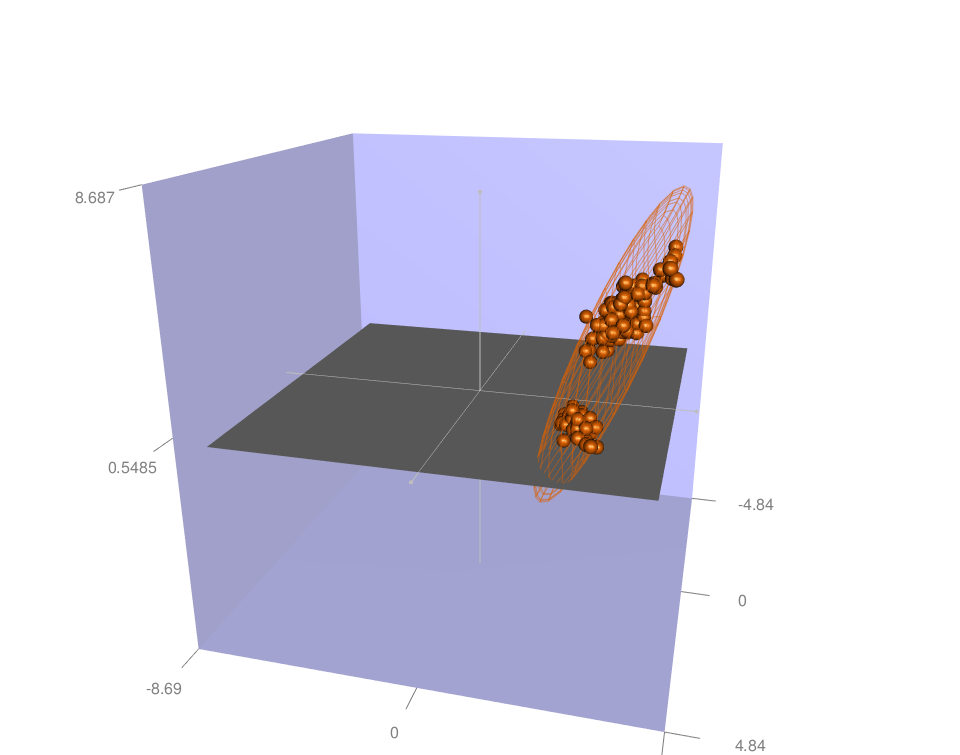
- Combine shade3d() and wired3d():
rgl_init()
rgl.spheres(x, y, z, r = 0.2, color = "#D95F02")
rgl_add_axes(x, y, z, show.bbox = TRUE)
# Compute and draw the ellipse of concentration
ellips <- ellipse3d(cov(cbind(x,y,z)),
            centre=c(mean(x), mean(y), mean(z)), level = 0.95)
shade3d(ellips, col = "#D95F02", alpha = 0.1, lit = FALSE)
wire3d(ellips, col = "#D95F02",  lit = FALSE)
aspect3d(1,1,1)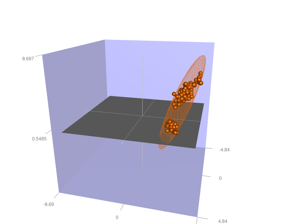
- Add ellipse for each group:
# Groups
groups <- iris$Species
levs <- levels(groups)
group.col <- c("red", "green", "blue")
# Plot observations
rgl_init()
rgl.spheres(x, y, z, r = 0.2,
            color = group.col[as.numeric(groups)])
rgl_add_axes(x, y, z, show.bbox = FALSE)
# Compute ellipse for each group
for (i in 1:length(levs)) {
    group <- levs[i]
    selected <- groups == group
    xx <- x[selected]; yy <- y[selected]; zz <- z[selected]
    ellips <- ellipse3d(cov(cbind(xx,yy,zz)),
              centre=c(mean(xx), mean(yy), mean(zz)), level = 0.95)
    shade3d(ellips, col = group.col[i], alpha = 0.1, lit = FALSE)
    # show group labels
    texts3d(mean(xx),mean(yy), mean(zz), text = group,
            col= group.col[i], cex = 2)
  }
aspect3d(1,1,1)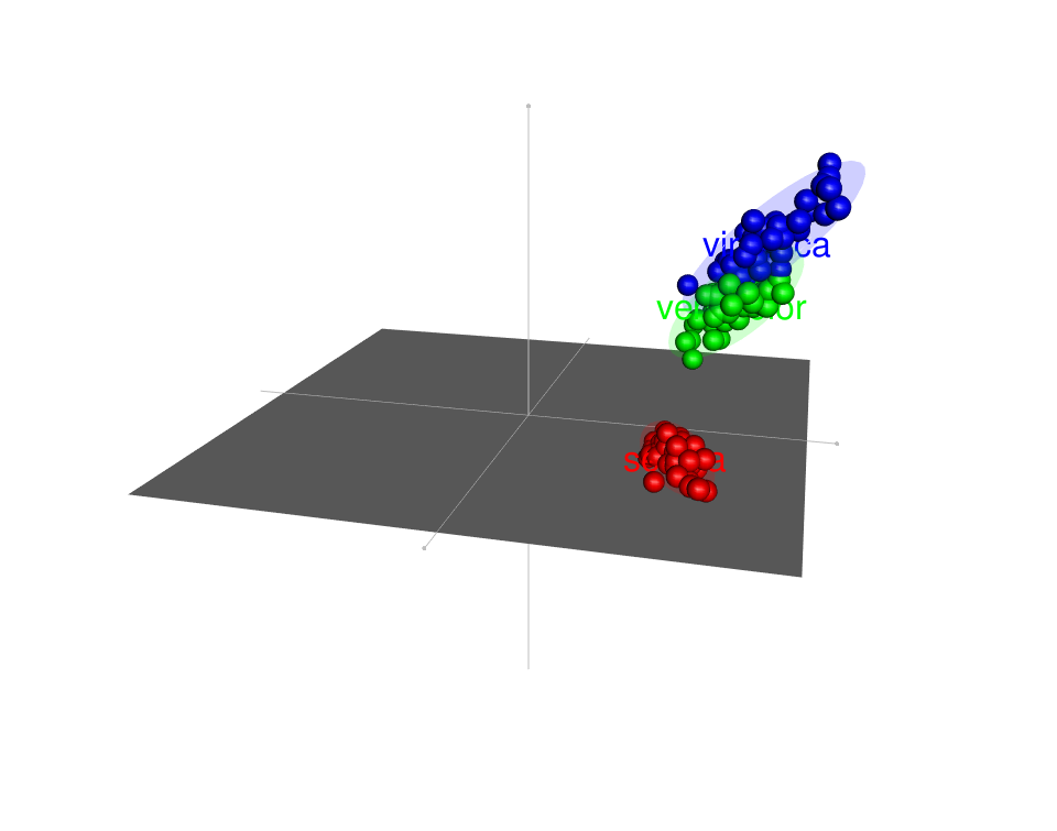
Regression plane
The function planes3d() or rgl.planes() can be used to add regression plane into 3D rgl plot:
rgl.planes(a, b = NULL, c = NULL, d = 0, ...)
planes3d(a, b = NULL, c = NULL, d = 0, ...)
planes3d() and rgl.planes() draw planes using the parameter ax + by + cz + d = 0.
- a, b, c: coordinates of the normal to the plane
- d: coordinates of the offset
Example of usage:
rgl_init()
rgl.spheres(x, y, z, r = 0.2, color = "#D95F02")
rgl_add_axes(x, y, z, show.bbox = FALSE)
aspect3d(1,1,1)
# Linear model
fit <- lm(z ~ x + y)
coefs <- coef(fit)
a <- coefs["x"]; b <- coefs["y"]; c <- -1
d <- coefs["(Intercept)"]
rgl.planes(a, b, c, d, alpha=0.2, color = "#D95F02")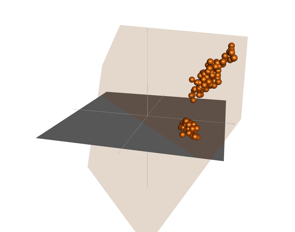
The regression plane above is very ugly. Let’s try to do a custom one. The steps below are followed:
- Use the function lm() to compute a linear regression model: ax + by + cz + d = 0
- Use the argument rgl.surface() to add a regression surface.
rgl_init()
rgl.spheres(x, y, z, r = 0.2, color = "#D95F02")
rgl_add_axes(x, y, z, show.bbox = FALSE)
aspect3d(1,1,1)
# Compute the linear regression (y = ax + bz + d)
fit <- lm(y ~ x + z)
# predict values on regular xz grid
grid.lines = 26
x.pred <- seq(min(x), max(x), length.out = grid.lines)
z.pred <- seq(min(z), max(z), length.out = grid.lines)
xz <- expand.grid( x = x.pred, z = z.pred)
y.pred <- matrix(predict(fit, newdata = xz),
                 nrow = grid.lines, ncol = grid.lines)
# Add regression surface
rgl.surface(x.pred, z.pred, y.pred, color = "steelblue",
                alpha = 0.5, lit = FALSE)
# Add grid lines
rgl.surface(x.pred, z.pred, y.pred, color = "black",
    alpha = 0.5, lit = FALSE, front = "lines", back = "lines")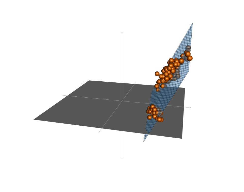
Create a movie of RGL scene
The function movie3d() can be used as follow:
movie3d(f, duration, dir = tempdir(), convert = TRUE)- f a function created using spin3d(axis)
- axis: the desired axis of rotation. Default value is c(0, 0, 1).
- duration : the duration of the animation
- dir: A directory in which to create temporary files for each frame of the movie
- convert: If TRUE, tries to convert the frames to a single GIF movie. It uses ImageMagick for the image conversion.
You should install ImageMagick (http://www.imagemagick.org/) to be able to create a movie from a list of png file.
rgl_init()
rgl.spheres(x, y, z, r = 0.2, color = "#D95F02")
rgl_add_axes(x, y, z, show.bbox = TRUE)
# Compute and draw the ellipse of concentration
ellips <- ellipse3d(cov(cbind(x,y,z)),
            centre=c(mean(x), mean(y), mean(z)), level = 0.95)
wire3d(ellips, col = "#D95F02",  lit = FALSE)
aspect3d(1,1,1)
# Create a movie
movie3d(spin3d(axis = c(0, 0, 1)), duration = 3,
        dir = getwd())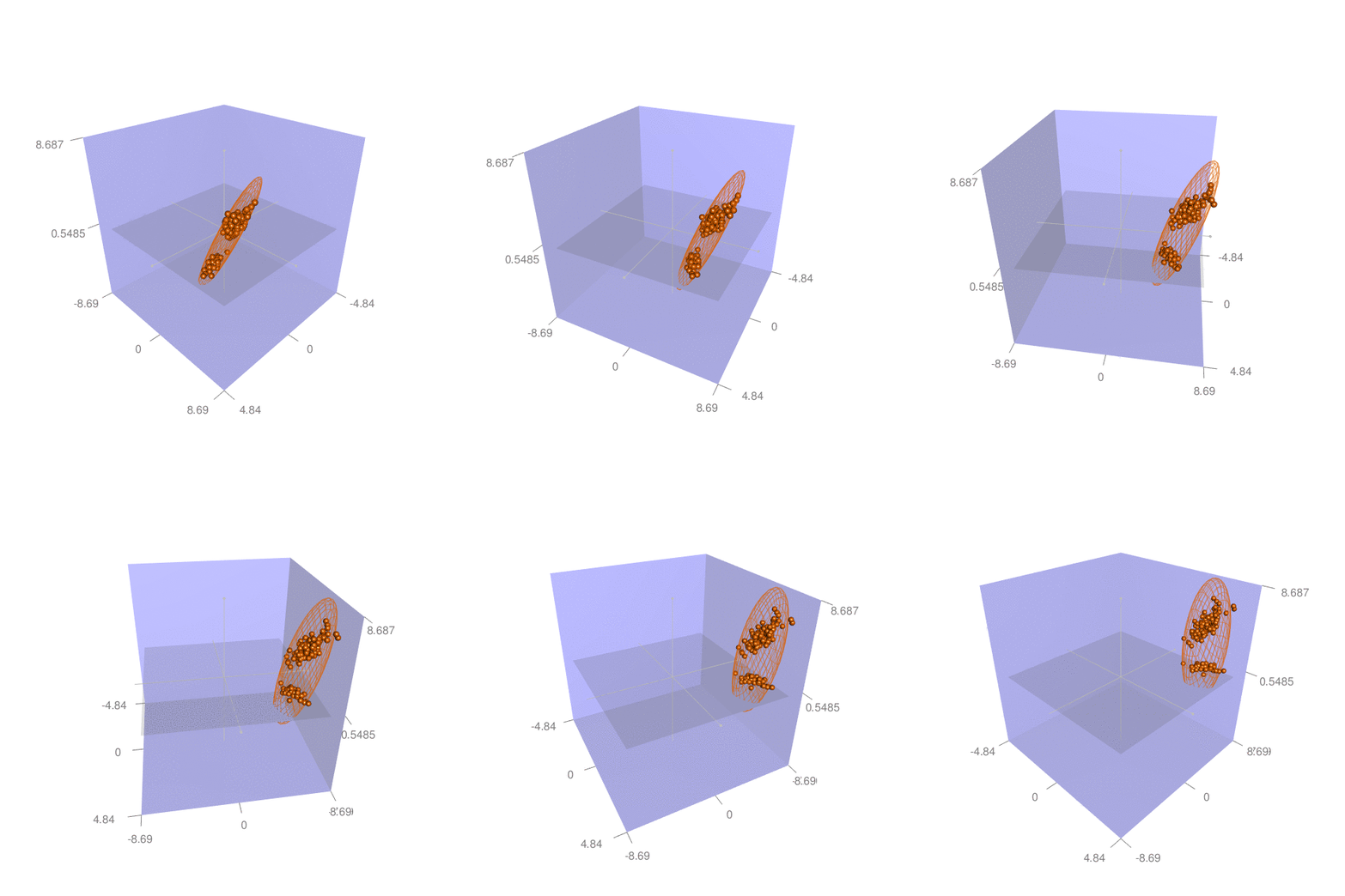
Export images as png or pdf
The plot can be saved as png or pdf.
- The function rgl.snapshot() is used to save the screenshot as png file:
rgl.snapshot(filename = "plot.png")- The function rgl.postscript() is used to save the screenshot to a file in ps, eps, tex, pdf, svg or pgf format:
rgl.postscript("plot.pdf",fmt="pdf")Example of usage:
rgl_init()
rgl.spheres(x, y, z, r = 0.2, color = "#D95F02")
rgl_add_axes(x, y, z, show.bbox = T)
aspect3d(1,1,1)
rg.snapshot("plot.png")
Export the plot into an interactive HTML file
The function writeWebGL() is used to write the current scene to HTML:
writeWebGL(dir = "webGL", filename = file.path(dir, "index.html"))- dir: Where to write the files
- filename: The file name to use for the main file
The R code below, writes a copy of the scene and then displays it in a browser:
rgl_init()
rgl.spheres(x, y, z, r = 0.2,
          color = get_colors(iris$Species))
rgl_add_axes(x, y, z, show.bbox = FALSE)
# This writes a copy into temporary directory 'webGL',
# and then displays it
browseURL(
  paste("file://", writeWebGL(dir=file.path(tempdir(), "webGL"),
  width=500), sep="")
  )
Select a rectangle in an RGL scene
The functions rgl.select3d() or select3d() can be used to select 3-dimensional regions.
They return a function f(x, y, z) which tests whether each of the points (x, y, z) is in the selected region.
The R code below, allows the user to select some points, and then redraw them in a different color:
rgl_init()
rgl.spheres(x, y, z, r = 0.2, color = "#D95F02")
rgl_add_axes(x, y, z, show.bbox = F)
aspect3d(1,1,1)
# Select a point
 f <- select3d()
 sel <- f(x,y,z)
rgl.clear("shapes")
# Redraw the points
rgl.spheres(x[!sel],y[!sel], z[!sel], r = 0.2, color = "#D95F02")
rgl.spheres(x[sel],y[sel], z[sel], r = 0.2, color = "green")
Identify points in a plot
The function identify3d() is used:
identify3d(x, y = NULL, z = NULL, labels, n)- x, y, z : Numeric vector specifying the coordinates of points. The arguments y and z are optional when:
- x is a matrix or a data frame containing at least 3 columns which will be used as the x, y and z coordinates.
- x is a formula of form zvar ~ xvar + yvar (see ?xyz.coords).
- labels an optional character vector giving labels for points
- n the maximum number of points to be identified
The function identify3d(), works similarly to the identify function in base graphics.
The R code below, allow the user to identify 5 points :
rgl_init()
rgl.spheres(x, y, z, r = 0.2, color = "#D95F02")
rgl_add_axes(x, y, z, show.bbox = F)
aspect3d(1,1,1)
rgl.material(color = "blue")
identify3d(x, y, z, labels = rownames(iris), n = 5)
Use the right button to select, the middle button to quit.
R3D Interface
The rgl package also includes a higher level interface called r3d. This interface is designed to act more like classic 2D R graphics.
The next sections describe how to make 3D graphics using the R3D interface.
3D Scatter plot
The function plot3d() is used:
## Default method
plot3d(x, y, z, xlab, ylab, zlab, type = "p", col,
        size, lwd, radius, add = FALSE, aspect = !add, ...)
## Method for class 'mesh3d'
plot3d(x, xlab = "x", ylab = "y", zlab = "z",
       type = c("shade", "wire", "dots"), add = FALSE, ...)
decorate3d(xlim, ylim, zlim,
  xlab = "x", ylab = "y", zlab = "z",
    box = TRUE, axes = TRUE, main = NULL, sub = NULL,
top = TRUE, aspect = FALSE, expand = 1.03, ...)- x, y, z: vectors of points to be drawn. Any reasonable way of defining the coordinates is acceptable. See the function xyz.coords for details
- xlab, yab, zlab: x, y and z axis labels
- type:
- For the default method: Allowed values are: ‘p’ for points, ‘s’ for spheres, ‘l’ for lines, ‘h’ for line segments from z = 0, and ‘n’ for nothing.
- For the mesh3d method, one of ‘shade’, ‘wire’, or ‘dots’
- col: the color to be used for plotted items
- size: size of points
- lwd: the line width for plotted item
- radius: the radius of sphere
- add: whether to add the points to an existing plot
- aspect: either a logical indicating whether to adjust the aspect ratio, or a new ratio
- …: additional parameters which will be passed to par3d, material3d or decorate3d
- box, axes: whether to draw a box and axes.
- main, sub: main title and subtitle
- top: whether to bring the window to the top when done
Note that, it’s recommended to use the function open3d() to initialize the *3d interface. However, in the following R code chunks, I’ll continue to use the custom function rgl_init().
Draw points:
rgl_init()
plot3d(x, y, z, col="blue", type ="p")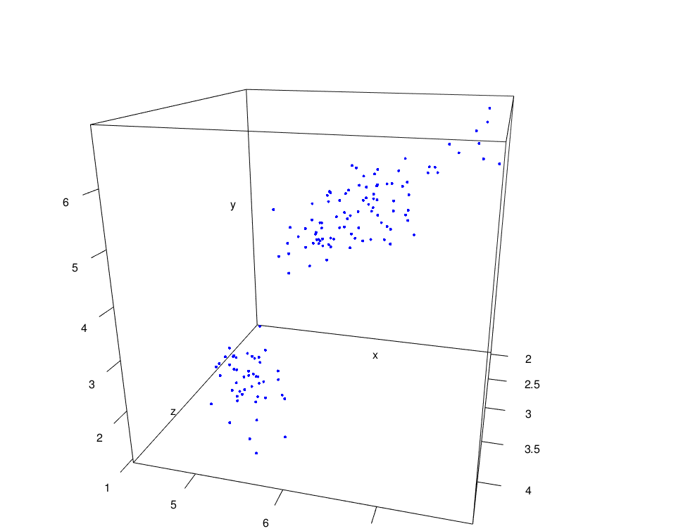
Remove the box and draw spheres:
rgl_init()
plot3d(x, y, z, col="blue", box = FALSE,
       type ="s", radius = 0.15)
To remove the axes, use the argument axes = FALSE.
Axis labels:
rgl_init()
plot3d(x, y, z, col="blue", box = FALSE,
       type ="s", radius = 0.15, xlab ="Sepal.Length",
       ylab = "Petal.Length", zlab = "Sepal.Width")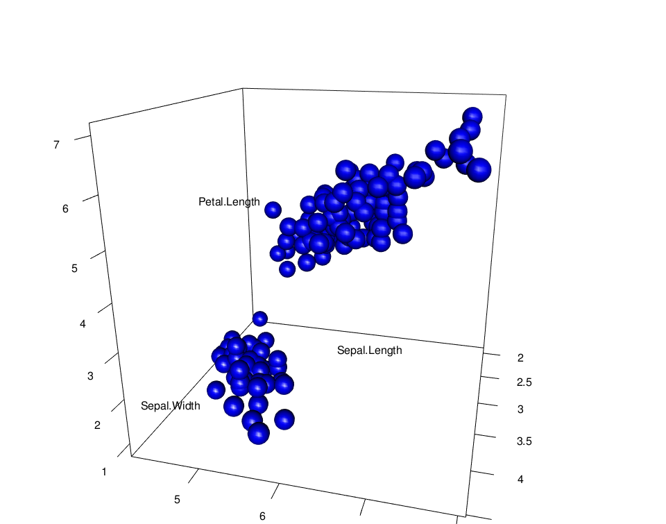
Add ellipse of concentration:
rgl_init()
plot3d(x, y, z, col="blue", box = FALSE,
       type ="s", radius = 0.15)
ellips <- ellipse3d(cov(cbind(x,y,z)),
            centre=c(mean(x), mean(y), mean(z)), level = 0.95)
plot3d(ellips, col = "blue", alpha = 0.2, add = TRUE, box = FALSE)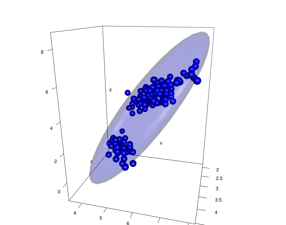
Change the ellipse type: possible values for the argument type = c(“shade”, “wire”, “dots”)
rgl_init()
plot3d(x, y, z, col="blue", box = FALSE,
       type ="s", radius = 0.15)
ellips <- ellipse3d(cov(cbind(x,y,z)),
            centre = c(mean(x), mean(y), mean(z)), level = 0.95)
plot3d(ellips, col = "blue", alpha = 0.5, add = TRUE, type = "wire")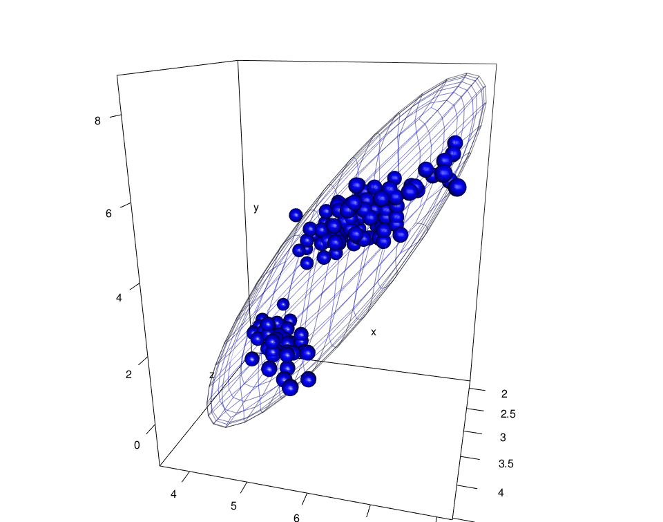
bbox3d(): Add bounding box decoration
rgl_init()
plot3d(x, y, z, col="blue", box = FALSE,
       type ="s", radius = 0.15)
# Add bounding box decoration
rgl.bbox(color=c("#333377","black"), emission="#333377",
         specular="#3333FF", shininess=5, alpha=0.8, nticks = 3 )
# Change the axis aspect ratios
aspect3d(1,1,1)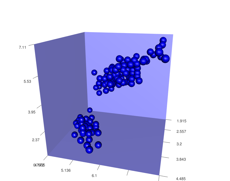
Some important functions
- open3d(): Open a new device
- Add a shape to the current scene:
- points3d(x, y, z, …)
- lines3d(x, y, z, …)
- segments3d(x, y, z, …)
- quads3d(x, y, z, …)
- texts3d(x, y, z, text): Adds text
- Draw boxes, axes and other text:
- axes3d(): Add standard axes
- title3d(main, sub, xlab, ylab, zlab): Add titles
- box3d(): Draws a box around the plot
- mtext3d(): to put a text in the plot margin(s)
RGL functions
Some important functions for managing RGL device are listed below:
Device management
| Functions | Description |
|---|---|
| rgl.open() | Opens a new device |
| rgl.close() | Closes the current device |
| rgl.cur() | Returns the ID of the active device |
| rgl.dev.list() | Returns all device IDs |
| rgl.set(which) | Set a device as active |
| rgl.quit() | Shutdown the RGL device system |
The equivalents in r3d interface:
Shape functions
Adds a shape node to the current scene.
| Functions | Description |
|---|---|
| rgl.points(x, y, z, …) | Draws a point at x, y and z |
| rgl.lines(x, y, z, …) | Draws line segments based on pairs of vertices (x = c(x1,x2), y = c(y1,y2), z = c(z1, z2)) |
| rgl.triangles(x, y, z, …) | Draws triangles with nodes (xi, yi, zi), i = 1, 2, 3 |
| rgl.quads(x, y, z) | Draws quads with nodes (xi, yi, zi), i = 1, 2, 3, 4 |
| rgl.spheres(x, y, z, r, …) | Draws spheres with center (x, y, z) and radius r |
| rgl.texts(x, y, z, text, …) | Adds text to the scene |
| rgl.surface(x, y, z, …) | Adds surface to the current scene. x and y are two vectors defining the grid. z is a matrix defining the height of each grid point |
Scene management
| Functions | Description |
|---|---|
| rgl.clear(type = “shapes”) | Clears the scene from the specified stack (“shapes”, “lights”, “bboxdeco”, “background”) |
| rgl.pop(type = “shapes”) | removes the last-added node from stack |
Setup the environment
| Functions | Description |
|---|---|
| rgl.viewpoint(theta, phi, fov, zoom, …) | Set the viewpoint orientation. theta and phi are the polar coordinates. fov is the field-of-view angle in degrees. zoom: zoom factor. |
| rgl.light(theta, phi, …) | Adds a light source to the scene |
| rgl.bg(…) | Setup the background environment of the scene |
| rgl.bbox(…) | Setup the bounding box decoration |
Appearance setup
| Functions | Description |
|---|---|
| rgl.material(…) | Set material properties for geometry appearance |
| aspect3d(x, y, z) | Set the aspect ratios of the x, y and z axes |
Export screenshot
| Functions | Description |
|---|---|
| rgl.snapshot(“plot.png”) | Saves a screenshot as png file |
| rgl.postscript(“plot.pdf”,fmt=“pdf”) | Saves the screenshot to a file in ps, eps, tex, pdf, svg or pgf format. |
Assign focus to an RGL window
Rgl.bringtotop(): ‘rgl.bringtotop’ brings the current RGL window to the front of the window stack (and gives it focus).
Infos
References:
- Daniel Alder et al., RGL: A R-library for 3D visualization with OpenGL, http://rgl.neoscientists.org/arc/doc/RGL_INTERFACE03.pdf
This analysis has been performed using R software (ver. 3.1.2) and rgl (ver. 0.93.1098)
Show me some love with the like buttons below... Thank you and please don't forget to share and comment below!!
Montrez-moi un peu d'amour avec les like ci-dessous ... Merci et n'oubliez pas, s'il vous plaît, de partager et de commenter ci-dessous!
Recommended for You!
Recommended for you
This section contains the best data science and self-development resources to help you on your path.
Books - Data Science
Our Books
- Practical Guide to Cluster Analysis in R by A. Kassambara (Datanovia)
- Practical Guide To Principal Component Methods in R by A. Kassambara (Datanovia)
- Machine Learning Essentials: Practical Guide in R by A. Kassambara (Datanovia)
- R Graphics Essentials for Great Data Visualization by A. Kassambara (Datanovia)
- GGPlot2 Essentials for Great Data Visualization in R by A. Kassambara (Datanovia)
- Network Analysis and Visualization in R by A. Kassambara (Datanovia)
- Practical Statistics in R for Comparing Groups: Numerical Variables by A. Kassambara (Datanovia)
- Inter-Rater Reliability Essentials: Practical Guide in R by A. Kassambara (Datanovia)
Others
- R for Data Science: Import, Tidy, Transform, Visualize, and Model Data by Hadley Wickham & Garrett Grolemund
- Hands-On Machine Learning with Scikit-Learn, Keras, and TensorFlow: Concepts, Tools, and Techniques to Build Intelligent Systems by Aurelien Géron
- Practical Statistics for Data Scientists: 50 Essential Concepts by Peter Bruce & Andrew Bruce
- Hands-On Programming with R: Write Your Own Functions And Simulations by Garrett Grolemund & Hadley Wickham
- An Introduction to Statistical Learning: with Applications in R by Gareth James et al.
- Deep Learning with R by François Chollet & J.J. Allaire
- Deep Learning with Python by François Chollet
Click to follow us on Facebook :
Comment this article by clicking on "Discussion" button (top-right position of this page)


