Cox Model Assumptions
Previously, we described the basic methods for analyzing survival data, as well as, the Cox proportional hazards methods to deal with the situation where several factors impact on the survival process.
In the current article, we continue the series by describing methods to evaluate the validity of the Cox model assumptions.
Note that, when used inappropriately, statistical models may give rise to misleading conclusions. Therefore, it’s important to check that a given model is an appropriate representation of the data.
Diagnostics for the Cox model
The Cox proportional hazards model makes sevral assumptions. Thus, it is important to assess whether a fitted Cox regression model adequately describes the data.
Here, we’ll disscuss three types of diagonostics for the Cox model:
- Testing the proportional hazards assumption.
- Examining influential observations (or outliers).
- Detecting nonlinearity in relationship between the log hazard and the covariates.
In order to check these model assumptions, Residuals method are used. The common residuals for the Cox model include:
- Schoenfeld residuals to check the proportional hazards assumption
- Martingale residual to assess nonlinearity
- Deviance residual (symmetric transformation of the Martinguale residuals), to examine influential observations
Assessing the validy of a Cox model in R
Installing and loading required R packages
We’ll use two R packages:
- survival for computing survival analyses
survminer for visualizing survival analysis results
Install the packages
install.packages(c("survival", "survminer"))- Load the packages
library("survival")
library("survminer")
Computing a Cox model
We’ll use the lung data sets and the coxph() function in the survival package.
To compute a Cox model, type this:
library("survival")
res.cox <- coxph(Surv(time, status) ~ age + sex + wt.loss, data =  lung)
res.cox
Call:
coxph(formula = Surv(time, status) ~ age + sex + wt.loss, data = lung)
coef exp(coef) se(coef) z p
age 0.02009 1.02029 0.00966 2.08 0.0377
sex -0.52103 0.59391 0.17435 -2.99 0.0028
wt.loss 0.00076 1.00076 0.00619 0.12 0.9024
Likelihood ratio test=14.7 on 3 df, p=0.00212
n= 214, number of events= 152
(14 observations deleted due to missingness)Testing proportional Hazards assumption
The proportional hazards (PH) assumption can be checked using statistical tests and graphical diagnostics based on the scaled Schoenfeld residuals.
In principle, the Schoenfeld residuals are independent of time. A plot that shows a non-random pattern against time is evidence of violation of the PH assumption.
The function cox.zph() [in the survival package] provides a convenient solution to test the proportional hazards assumption for each covariate included in a Cox refression model fit.
For each covariate, the function cox.zph() correlates the corresponding set of scaled Schoenfeld residuals with time, to test for independence between residuals and time. Additionally, it performs a global test for the model as a whole.
The proportional hazard assumption is supported by a non-significant relationship between residuals and time, and refuted by a significant relationship.
To illustrate the test, we start by computing a Cox regression model using the lung data set [in survival package]:
library("survival")
res.cox <- coxph(Surv(time, status) ~ age + sex + wt.loss, data =  lung)
res.cox
Call:
coxph(formula = Surv(time, status) ~ age + sex + wt.loss, data = lung)
coef exp(coef) se(coef) z p
age 0.02009 1.02029 0.00966 2.08 0.0377
sex -0.52103 0.59391 0.17435 -2.99 0.0028
wt.loss 0.00076 1.00076 0.00619 0.12 0.9024
Likelihood ratio test=14.7 on 3 df, p=0.00212
n= 214, number of events= 152
(14 observations deleted due to missingness)To test for the proportional-hazards (PH) assumption, type this:
test.ph <- cox.zph(res.cox)
test.ph
rho chisq p
age -0.0483 0.378 0.538
sex 0.1265 2.349 0.125
wt.loss 0.0126 0.024 0.877
GLOBAL NA 2.846 0.416From the output above, the test is not statistically significant for each of the covariates, and the global test is also not statistically significant. Therefore, we can assume the proportional hazards.
It’s possible to do a graphical diagnostic using the function ggcoxzph() [in the survminer package], which produces, for each covariate, graphs of the scaled Schoenfeld residuals against the transformed time.
ggcoxzph(test.ph)
Cox Model Assumptions
In the figure above, the solid line is a smoothing spline fit to the plot, with the dashed lines representing a +/- 2-standard-error band around the fit.
Note that, systematic departures from a horizontal line are indicative of non-proportional hazards, since proportional hazards assumes that estimates \(\beta_1, \beta_2, \beta_3\) do not vary much over time.
From the graphical inspection, there is no pattern with time. The assumption of proportional hazards appears to be supported for the covariates sex (which is, recall, a two-level factor, accounting for the two bands in the graph), wt.loss and age.
Another graphical methods for checking proportional hazards is to plot log(-log(S(t))) vs. t or log(t) and look for parallelism. This can be done only for categorical covariates.
A violations of proportional hazards assumption can be resolved by:
- Adding covariate*time interaction
- Stratification
Stratification is usefull for “nuisance” confounders, where you do not care to estimate the effect. You cannot examine the effects of the stratification variable (John Fox & Sanford Weisberg).
To read more about how to accomodate with non-proportional hazards, read the following articles:
- Jadwiga Borucka, PAREXEL, Warsaw, Poland. Extensions of cox model for non-proportional hazards purpose. 2013.
- John Fox & Sanford Weisberg. Cox Proportional-Hazards Regression for Survival Data in R.
- Max Gordon. Dealing with non-proportional hazards in R. March 29, 2016.
Testing influential observations
To test influential observations or outliers, we can visualize either:
- the deviance residuals or
- the dfbeta values
The function ggcoxdiagnostics()[in survminer package] provides a convenient solution for checkind influential observations. The simplified format is as follow:
ggcoxdiagnostics(fit, type = , linear.predictions = TRUE)- fit: an object of class coxph.object
- type: the type of residuals to present on Y axis. Allowed values include one of c(“martingale”, “deviance”, “score”, “schoenfeld”, “dfbeta”, “dfbetas”, “scaledsch”, “partial”).
- linear.predictions: a logical value indicating whether to show linear predictions for observations (TRUE) or just indexed of observations (FALSE) on X axis.
Specifying the argument type = “dfbeta”, plots the estimated changes in the regression coefficients upon deleting each observation in turn; likewise, type=“dfbetas” produces the estimated changes in the coefficients divided by their standard errors.
For example:
ggcoxdiagnostics(res.cox, type = "dfbeta",
                 linear.predictions = FALSE, ggtheme = theme_bw())
Cox Model Assumptions
(Index plots of dfbeta for the Cox regression of time to death on age, sex and wt.loss)
The above index plots show that comparing the magnitudes of the largest dfbeta values to the regression coefficients suggests that none of the observations is terribly influential individually, even though some of the dfbeta values for age and wt.loss are large compared with the others.
It’s also possible to check outliers by visualizing the deviance residuals. The deviance residual is a normalized transform of the martingale residual. These residuals should be roughtly symmetrically distributed about zero with a standard deviation of 1.
- Positive values correspond to individuals that “died too soon” compared to expected survival times.
- Negative values correspond to individual that “lived too long”.
- Very large or small values are outliers, which are poorly predicted by the model.
Example of deviance residuals:
ggcoxdiagnostics(res.cox, type = "deviance",
                 linear.predictions = FALSE, ggtheme = theme_bw())
Cox Model Assumptions
The pattern looks fairly symmetric around 0.
Testing non linearity
Often, we assume that continuous covariates have a linear form. However, this assumption should be checked.
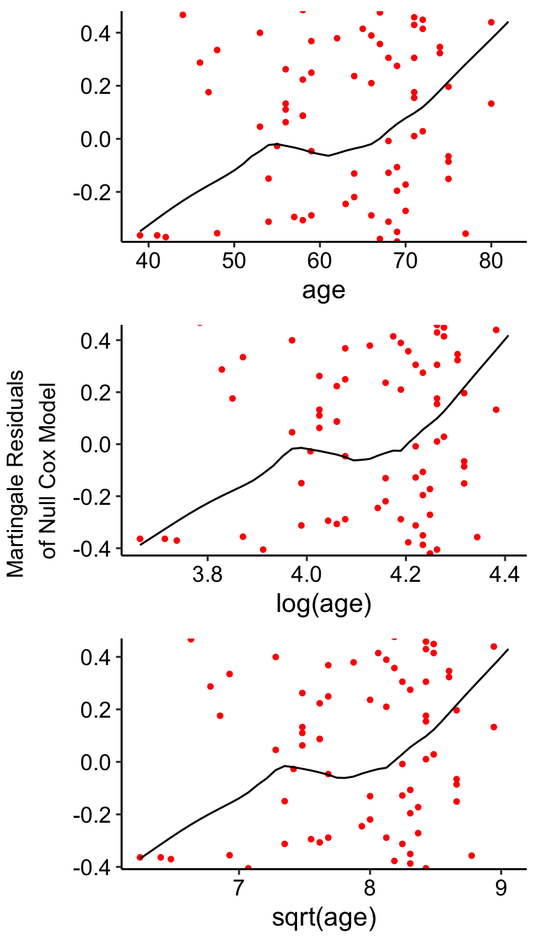
Plotting the Martingale residuals against continuous covariates is a common approach used to detect nonlinearity or, in other words, to assess the functional form of a covariate. For a given continuous covariate, patterns in the plot may suggest that the variable is not properly fit.
Nonlinearity is not an issue for categorical variables, so we only examine plots of martingale residuals and partial residuals against a continuous variable.
Martingale residuals may present any value in the range (-INF, +1):
- A value of martinguale residuals near 1 represents individuals that “died too soon”,
- and large negative values correspond to individuals that “lived too long”.
To assess the functional form of a continuous variable in a Cox proportional hazards model, we’ll use the function ggcoxfunctional() [in the survminer R package].
The function ggcoxfunctional() displays graphs of continuous covariates against martingale residuals of null cox proportional hazards model. This might help to properly choose the functional form of continuous variable in the Cox model. Fitted lines with lowess function should be linear to satisfy the Cox proportional hazards model assumptions.
For example, to assess the functional forme of age, type this:
ggcoxfunctional(Surv(time, status) ~ age + log(age) + sqrt(age), data = lung)
Cox Model Assumptions
It appears that, nonlinearity is slightly here.
Summary
We described how to assess the valididy of the Cox model assumptions using the survival and survminer packages.
Infos
This analysis has been performed using R software (ver. 3.3.2).
Show me some love with the like buttons below... Thank you and please don't forget to share and comment below!!
Montrez-moi un peu d'amour avec les like ci-dessous ... Merci et n'oubliez pas, s'il vous plaît, de partager et de commenter ci-dessous!
Recommended for You!
Recommended for you
This section contains the best data science and self-development resources to help you on your path.
Books - Data Science
Our Books
- Practical Guide to Cluster Analysis in R by A. Kassambara (Datanovia)
- Practical Guide To Principal Component Methods in R by A. Kassambara (Datanovia)
- Machine Learning Essentials: Practical Guide in R by A. Kassambara (Datanovia)
- R Graphics Essentials for Great Data Visualization by A. Kassambara (Datanovia)
- GGPlot2 Essentials for Great Data Visualization in R by A. Kassambara (Datanovia)
- Network Analysis and Visualization in R by A. Kassambara (Datanovia)
- Practical Statistics in R for Comparing Groups: Numerical Variables by A. Kassambara (Datanovia)
- Inter-Rater Reliability Essentials: Practical Guide in R by A. Kassambara (Datanovia)
Others
- R for Data Science: Import, Tidy, Transform, Visualize, and Model Data by Hadley Wickham & Garrett Grolemund
- Hands-On Machine Learning with Scikit-Learn, Keras, and TensorFlow: Concepts, Tools, and Techniques to Build Intelligent Systems by Aurelien Géron
- Practical Statistics for Data Scientists: 50 Essential Concepts by Peter Bruce & Andrew Bruce
- Hands-On Programming with R: Write Your Own Functions And Simulations by Garrett Grolemund & Hadley Wickham
- An Introduction to Statistical Learning: with Applications in R by Gareth James et al.
- Deep Learning with R by François Chollet & J.J. Allaire
- Deep Learning with Python by François Chollet
Click to follow us on Facebook :
Comment this article by clicking on "Discussion" button (top-right position of this page)


