HCPC - Hierarchical Clustering on Principal Components: Essentials
Clustering is one of the important data mining methods for discovering knowledge in multivariate data sets. The goal is to identify groups (i.e. clusters) of similar objects within a data set of interest. To learn more about clustering, you can read our book entitled “Practical Guide to Cluster Analysis in R” (https://goo.gl/DmJ5y5).
Briefly, the two most common clustering strategies are:
- Hierarchical clustering, used for identifying groups of similar observations in a data set.
- Partitioning clustering such as k-means algorithm, used for splitting a data set into several groups.
The HCPC (Hierarchical Clustering on Principal Components) approach allows us to combine the three standard methods used in multivariate data analyses (Husson, Josse, and J. 2010):
- Principal component methods (PCA, CA, MCA, FAMD, MFA),
- Hierarchical clustering and
- Partitioning clustering, particularly the k-means method.
This chapter describes WHY and HOW to combine principal components and clustering methods. Finally, we demonstrate how to compute and visualize HCPC using R software.
Contents:
Why HCPC
Combining principal component methods and clustering methods are useful in at least three situations.
Case 1: Continuous variables
In the situation where you have a multidimensional data set containing multiple continuous variables, the principal component analysis (PCA) can be used to reduce the dimension of the data into few continuous variables containing the most important information in the data. Next, you can perform cluster analysis on the PCA results.
The PCA step can be considered as a denoising step which can lead to a more stable clustering. This might be very useful if you have a large data set with multiple variables, such as in gene expression data.
Case 2: Clustering on categorical data
In order to perform clustering analysis on categorical data, the correspondence analysis (CA, for analyzing contingency table) and the multiple correspondence analysis (MCA, for analyzing multidimensional categorical variables) can be used to transform categorical variables into a set of few continuous variables (the principal components). The cluster analysis can be then applied on the (M)CA results.
In this case, the (M)CA method can be considered as pre-processing steps which allow to compute clustering on categorical data.
Case 3: Clustering on mixed data
When you have a mixed data of continuous and categorical variables, you can first perform FAMD (factor analysis of mixed data) or MFA (multiple factor analysis). Next, you can apply cluster analysis on the FAMD/MFA outputs.
Algorithm of the HCPC method
The algorithm of the HCPC method, as implemented in the FactoMineR package, can be summarized as follow:
Compute principal component methods: PCA, (M)CA or MFA depending on the types of variables in the data set and the structure of the data set. At this step, you can choose the number of dimensions to be retained in the output by specifying the argument ncp. The default value is 5.Compute hierarchical clustering: Hierarchical clustering is performed using the Ward’s criterion on the selected principal components. Ward criterion is used in the hierarchical clustering because it is based on the multidimensional variance like principal component analysis.Choose the number of clusters based on the hierarchical tree: An initial partitioning is performed by cutting the hierarchical tree.Perform K-means clusteringto improve the initial partition obtained from hierarchical clustering. The final partitioning solution, obtained after consolidation with k-means, can be (slightly) different from the one obtained with the hierarchical clustering.
Computation
R packages
We’ll use two R packages: i) FactoMineR for computing HCPC and ii) factoextra for visualizing the results.
To install the packages, type this:
install.packages(c("FactoMineR", "factoextra"))After the installation, load the packages as follow:
library(factoextra)
library(FactoMineR)
R function
The function HCPC() [in FactoMineR package] can be used to compute hierarchical clustering on principal components.
A simplified format is:
HCPC(res, nb.clust = 0, min = 3, max = NULL, graph = TRUE)res: Either the result of a factor analysis or a data frame.nb.clust: an integer specifying the number of clusters. Possible values are:0: the tree is cut at the level the user clicks on-1: the tree is automatically cut at the suggested levelAny positive integer: the tree is cut with nb.clusters clusters
min, max: the minimum and the maximum number of clusters to be generated, respectivelygraph: if TRUE, graphics are displayed
Case of continuous variables
We start by computing again the principal component analysis (PCA). The argument ncp = 3 is used in the function PCA() to keep only the first three principal components. Next, the HCPC is applied on the result of the PCA.
library(FactoMineR)
# Compute PCA with ncp = 3
res.pca <- PCA(USArrests, ncp = 3, graph = FALSE)
# Compute hierarchical clustering on principal components
res.hcpc <- HCPC(res.pca, graph = FALSE)
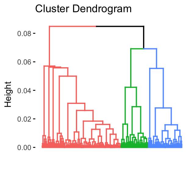
To visualize the dendrogram generated by the hierarchical clustering, we’ll use the function fviz_dend() [factoextra package]:
fviz_dend(res.hcpc,
          cex = 0.7,                     # Label size
          palette = "jco",               # Color palette see ?ggpubr::ggpar
          rect = TRUE, rect_fill = TRUE, # Add rectangle around groups
          rect_border = "jco",           # Rectangle color
          labels_track_height = 0.8      # Augment the room for labels
          )
The dendrogram suggests 4 clusters solution.
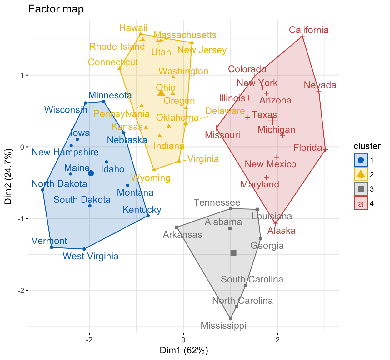
It’s possible to visualize individuals on the principal component map and to color individuals according to the cluster they belong to. The function fviz_cluster() [in factoextra] can be used to visualize individuals clusters.
fviz_cluster(res.hcpc,
             repel = TRUE,            # Avoid label overlapping
             show.clust.cent = TRUE, # Show cluster centers
             palette = "jco",         # Color palette see ?ggpubr::ggpar
             ggtheme = theme_minimal(),
             main = "Factor map"
             )
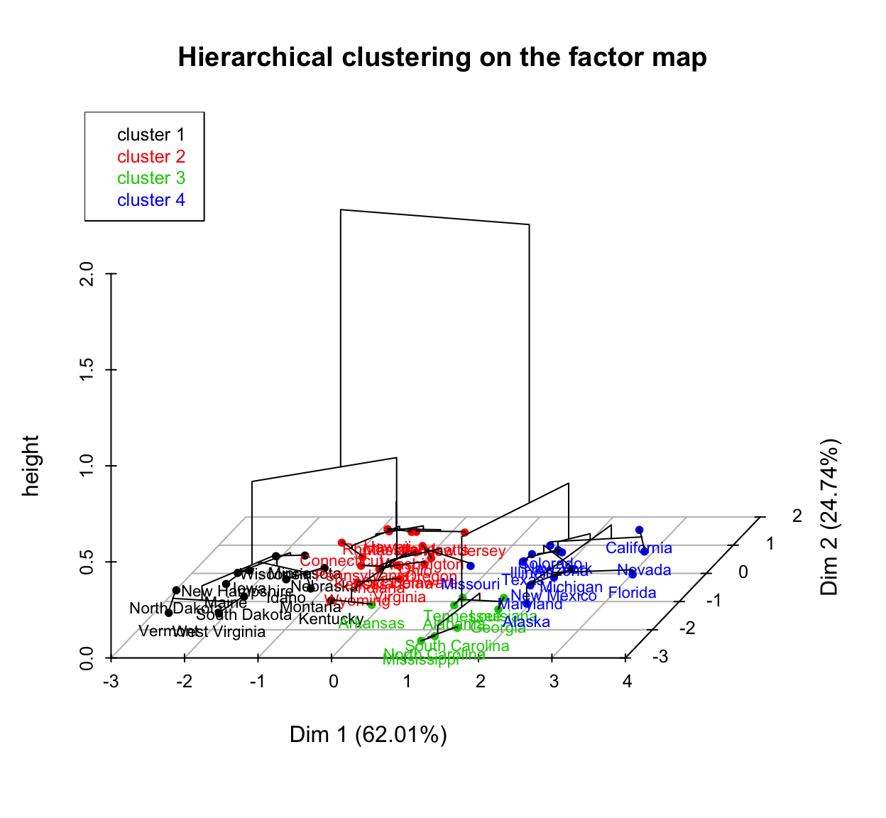
You can also draw a three dimensional plot combining the hierarchical clustering and the factorial map using the R base function plot():
# Principal components + tree
plot(res.hcpc, choice = "3D.map")
The function HCPC() returns a list containing:
data.clust: The original data with a supplementary column called class containing the partition.desc.var: The variables describing clustersdesc.ind: The more typical individuals of each clusterdesc.axes: The axes describing clusters
To display the original data with cluster assignments, type this:
head(res.hcpc$data.clust, 10)## Murder Assault UrbanPop Rape clust
## Alabama 13.2 236 58 21.2 3
## Alaska 10.0 263 48 44.5 4
## Arizona 8.1 294 80 31.0 4
## Arkansas 8.8 190 50 19.5 3
## California 9.0 276 91 40.6 4
## Colorado 7.9 204 78 38.7 4
## Connecticut 3.3 110 77 11.1 2
## Delaware 5.9 238 72 15.8 2
## Florida 15.4 335 80 31.9 4
## Georgia 17.4 211 60 25.8 3In the table above, the last column contains the cluster assignments.
To display quantitative variables that describe the most each cluster, type this:
res.hcpc$desc.var$quantiHere, we show only some columns of interest: “Mean in category”, “Overall Mean”, “p.value”
## $`1`
##          Mean in category Overall mean  p.value
## UrbanPop             52.1        65.54 9.68e-05
## Murder                3.6         7.79 5.57e-05
## Rape                 12.2        21.23 5.08e-05
## Assault              78.5       170.76 3.52e-06
##
## $`2`
##          Mean in category Overall mean p.value
## UrbanPop            73.88        65.54 0.00522
## Murder               5.66         7.79 0.01759
##
## $`3`
##          Mean in category Overall mean  p.value
## Murder               13.9         7.79 1.32e-05
## Assault             243.6       170.76 6.97e-03
## UrbanPop             53.8        65.54 1.19e-02
##
## $`4`
##          Mean in category Overall mean  p.value
## Rape                 33.2        21.23 8.69e-08
## Assault             257.4       170.76 1.32e-05
## UrbanPop             76.0        65.54 2.45e-03
## Murder               10.8         7.79 3.58e-03
From the output above, it can be seen that:
-
the variables UrbanPop, Murder, Rape and Assault are most significantly associated with the cluster 1. For example, the mean value of the Assault variable in cluster 1 is 78.53 which is less than it’s overall mean (170.76) across all clusters. Therefore, It can be conclude that the cluster 1 is characterized by a low rate of Assault compared to all clusters.
-
the variables UrbanPop and Murder are most significantly associated with the cluster 2.
…and so on …
Similarly, to show principal dimensions that are the most associated with clusters, type this:
res.hcpc$desc.axes$quanti## $`1`
## Mean in category Overall mean p.value
## Dim.1 -1.96 -5.64e-16 2.27e-07
##
## $`2`
## Mean in category Overall mean p.value
## Dim.2 0.743 -5.37e-16 0.000336
##
## $`3`
## Mean in category Overall mean p.value
## Dim.1 1.061 -5.64e-16 3.96e-02
## Dim.3 0.397 3.54e-17 4.25e-02
## Dim.2 -1.477 -5.37e-16 5.72e-06
##
## $`4`
## Mean in category Overall mean p.value
## Dim.1 1.89 -5.64e-16 6.15e-07The results above indicate that, individuals in clusters 1 and 4 have high coordinates on axes 1. Individuals in cluster 2 have high coordinates on the second axis. Individuals who belong to the third cluster have high coordinates on axes 1, 2 and 3.
Finally, representative individuals of each cluster can be extracted as follow:
res.hcpc$desc.ind$para## Cluster: 1
## Idaho South Dakota Maine Iowa New Hampshire
## 0.367 0.499 0.501 0.553 0.589
## --------------------------------------------------------
## Cluster: 2
## Ohio Oklahoma Pennsylvania Kansas Indiana
## 0.280 0.505 0.509 0.604 0.710
## --------------------------------------------------------
## Cluster: 3
## Alabama South Carolina Georgia Tennessee Louisiana
## 0.355 0.534 0.614 0.852 0.878
## --------------------------------------------------------
## Cluster: 4
## Michigan Arizona New Mexico Maryland Texas
## 0.325 0.453 0.518 0.901 0.924For each cluster, the top 5 closest individuals to the cluster center is shown. The distance between each individual and the cluster center is provided. For example, representative individuals for cluster 1 include: Idaho, South Dakota, Maine, Iowa and New Hampshire.
Case of categorical variables
For categorical variables, compute CA or MCA and then apply the function HCPC() on the results as described above.
Here, we’ll use the tea data [in FactoMineR] as demo data set: Rows represent the individuals and columns represent categorical variables.
We start, by performing an MCA on the individuals. We keep the first 20 axes of the MCA which retain 87% of the information.
# Loading data
library(FactoMineR)
data(tea)
# Performing MCA
res.mca <- MCA(tea,
               ncp = 20,            # Number of components kept
               quanti.sup = 19,     # Quantitative supplementary variables
               quali.sup = c(20:36), # Qualitative supplementary variables
               graph=FALSE)
Next, we apply hierarchical clustering on the results of the MCA:
res.hcpc <- HCPC (res.mca, graph = FALSE, max = 3)The results can be visualized as follow:
# Dendrogram
fviz_dend(res.hcpc, show_labels = FALSE)
# Individuals facor map
fviz_cluster(res.hcpc, geom = "point", main = "Factor map")

As mentioned above, clusters can be described by i) variables and/or categories, ii) principal axes and iii) individuals. In the example below, we display only a subset of the results.
- Description by variables and categories
# Description by variables
res.hcpc$desc.var$test.chi2
## p.value df
## where 8.47e-79 4
## how 3.14e-47 4
## price 1.86e-28 10
## tearoom 9.62e-19 2# Description by variable categories
res.hcpc$desc.var$category## $`1`
## Cla/Mod Mod/Cla Global p.value
## where=chain store 85.9 93.8 64.0 2.09e-40
## how=tea bag 84.1 81.2 56.7 1.48e-25
## tearoom=Not.tearoom 70.7 97.2 80.7 1.08e-18
## price=p_branded 83.2 44.9 31.7 1.63e-09
##
## $`2`
## Cla/Mod Mod/Cla Global p.value
## where=tea shop 90.0 84.4 10.0 3.70e-30
## how=unpackaged 66.7 75.0 12.0 5.35e-20
## price=p_upscale 49.1 81.2 17.7 2.39e-17
## Tea=green 27.3 28.1 11.0 4.44e-03
##
## $`3`
## Cla/Mod Mod/Cla Global p.value
## where=chain store+tea shop 85.9 72.8 26.0 5.73e-34
## how=tea bag+unpackaged 67.0 68.5 31.3 1.38e-19
## tearoom=tearoom 77.6 48.9 19.3 1.25e-16
## pub=pub 63.5 43.5 21.0 1.13e-09The variables that characterize the most the clusters are the variables “where” and “how”. Each cluster is characterized by a category of the variables “where” and “how”. For example, individuals who belong to the first cluster buy tea as tea bag in chain stores.
- Description by principal components
res.hcpc$desc.axes- Description by individuals
res.hcpc$desc.ind$paraSummary
We described how to compute hierarchical clustering on principal components (HCPC). This approach is useful in situations, including:
When you have a large data set containing continuous variables, a principal component analysis can be used to reduce the dimension of the data before the hierarchical clustering analysis.
When you have a data set containing categorical variables, a (Multiple)Correspondence analysis can be used to transform the categorical variables into few continuous principal components, which can be used as the input of the cluster analysis.
We used the FactoMineR package to compute the HCPC and the factoextra R package for ggplot2-based elegant data visualization.
Further reading
- Practical guide to cluster analysis in R (Book). https://goo.gl/DmJ5y5
- HCPC: Hierarchical Clustering on Principal Components (Videos). https://goo.gl/jdYGoK
References
Husson, François, J. Josse, and Pagès J. 2010. “Principal Component Methods - Hierarchical Clustering - Partitional Clustering: Why Would We Need to Choose for Visualizing Data?” Unpublished Data. https://www.sthda.com/english/upload/hcpc_husson_josse.pdf.


