Before applying any clustering method on your data, it’s important to evaluate whether the data sets contains meaningful clusters (i.e.: non-random structures) or not. If yes, then how many clusters are there. This process is defined as the assessing of clustering tendency or the feasibility of the clustering analysis.
A big issue, in cluster analysis, is that clustering methods will return clusters even if the data does not contain any clusters. In other words, if you blindly apply a clustering method on a data set, it will divide the data into clusters because that is what it supposed to do.
In this chapter, we start by describing why we should evaluate the clustering tendency before applying any clustering method on a data. Next, we provide statistical and visual methods for assessing the clustering tendency.
Contents:
Related Book
Practical Guide to Cluster Analysis in RRequired R packages
- factoextra for data visualization
- clustertend for statistical assessment clustering tendency
To install the two packages, type this:
install.packages(c("factoextra", "clustertend"))Data preparation
We’ll use two data sets:
- the built-in R data set iris.
- and a random data set generated from the iris data set.
The iris data sets look like this:
head(iris, 3)## Sepal.Length Sepal.Width Petal.Length Petal.Width Species
## 1 5.1 3.5 1.4 0.2 setosa
## 2 4.9 3.0 1.4 0.2 setosa
## 3 4.7 3.2 1.3 0.2 setosaWe start by excluding the column “Species” at position 5
# Iris data set
df <- iris[, -5]
# Random data generated from the iris data set
random_df <- apply(df, 2,
                function(x){runif(length(x), min(x), (max(x)))})
random_df <- as.data.frame(random_df)
# Standardize the data sets
df <- iris.scaled <- scale(df)
random_df <- scale(random_df)
Visual inspection of the data
We start by visualizing the data to assess whether they contains any meaningful clusters.
As the data contain more than two variables, we need to reduce the dimensionality in order to plot a scatter plot. This can be done using principal component analysis (PCA) algorithm (R function: prcomp()). After performing PCA, we use the function fviz_pca_ind() [factoextra R package] to visualize the output.
The iris and the random data sets can be illustrated as follow:
library("factoextra")
# Plot faithful data set
fviz_pca_ind(prcomp(df), title = "PCA - Iris data",
             habillage = iris$Species,  palette = "jco",
             geom = "point", ggtheme = theme_classic(),
             legend = "bottom")

# Plot the random df
fviz_pca_ind(prcomp(random_df), title = "PCA - Random data",
             geom = "point", ggtheme = theme_classic())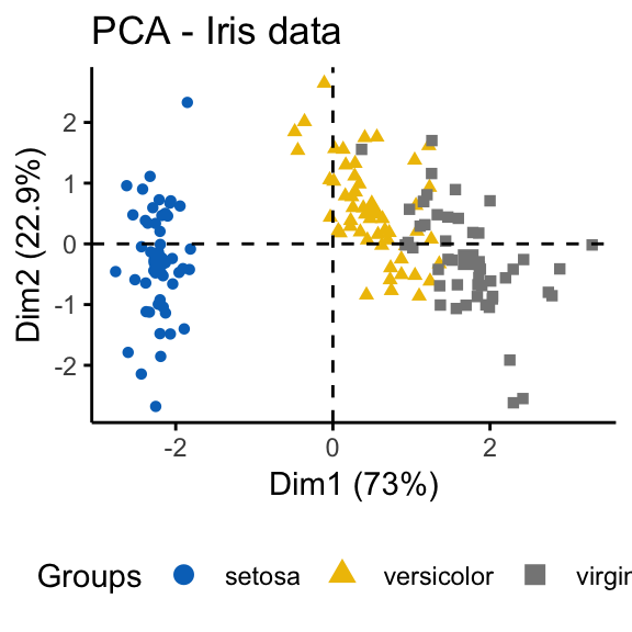
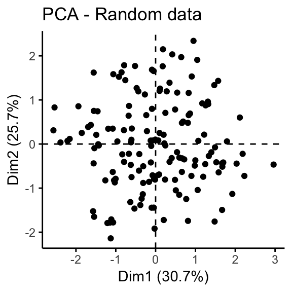
It can be seen that the iris data set contains 3 real clusters. However the randomly generated data set doesn’t contain any meaningful clusters.
Why assessing clustering tendency?
In order to illustrate why it’s important to assess cluster tendency, we start by computing k-means clustering and hierarchical clustering on the two data sets (the real and the random data).
The function fviz_cluster() and fviz_dend() [in factoextra R package] will be used to visualize the results.
library(factoextra)
set.seed(123)
# K-means on iris dataset
km.res1 <- kmeans(df, 3)
fviz_cluster(list(data = df, cluster = km.res1$cluster),
             ellipse.type = "norm", geom = "point", stand = FALSE,
             palette = "jco", ggtheme = theme_classic())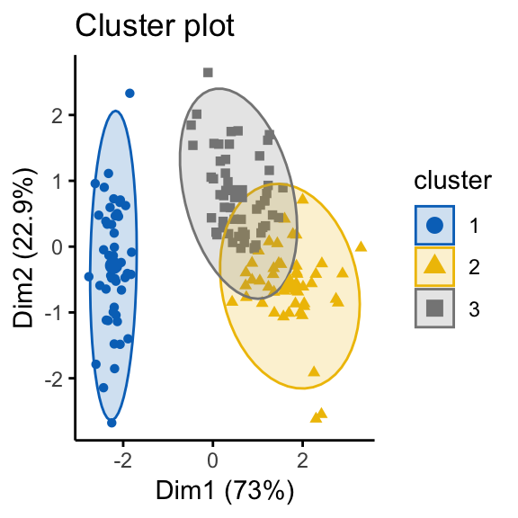
# K-means on the random dataset
km.res2 <- kmeans(random_df, 3)
fviz_cluster(list(data = random_df, cluster = km.res2$cluster),
             ellipse.type = "norm", geom = "point", stand = FALSE,
             palette = "jco", ggtheme = theme_classic())

# Hierarchical clustering on the random dataset
fviz_dend(hclust(dist(random_df)), k = 3, k_colors = "jco",
          as.ggplot = TRUE, show_labels = FALSE)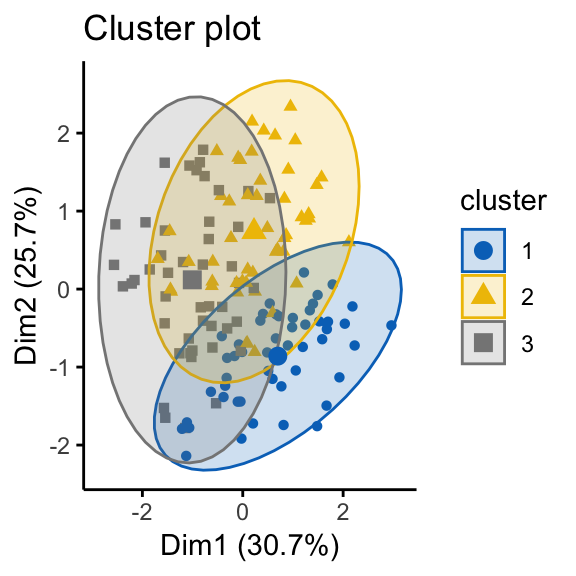
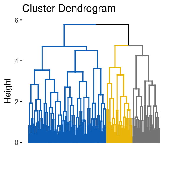
It can be seen that the k-means algorithm and the hierarchical clustering impose a classification on the random uniformly distributed data set even if there are no meaningful clusters present in it. This is why, clustering tendency assessment methods should be used to evaluate the validity of clustering analysis. That is, whether a given data set contains meaningful clusters.
Methods for assessing clustering tendency
In this section, we’ll describe two methods for evaluating the clustering tendency: i) a statistical (Hopkins statistic) and ii) a visual methods (Visual Assessment of cluster Tendency (VAT) algorithm).
Statistical methods
The Hopkins statistic (Lawson and Jurs 1990) is used to assess the clustering tendency of a data set by measuring the probability that a given data set is generated by a uniform data distribution. In other words, it tests the spatial randomness of the data.
For example, let D be a real data set. The Hopkins statistic can be calculated as follow:
- Sample uniformly \(n\) points (\(p_1\),…, \(p_n\)) from D.
- Compute the distance, \(x_i\), from each real point to each nearest neighbor: For each point \(p_i \in D\), find it’s nearest neighbor \(p_j\); then compute the distance between \(p_i\) and \(p_j\) and denote it as \(x_i = dist(p_i, p_j)\)
- Generate a simulated data set (\(random_D\)) drawn from a random uniform distribution with \(n\) points (\(q_1\),…, \(q_n\)) and the same variation as the original real data set D.
- Compute the distance, \(y_i\) from each artificial point to the nearest real data point: For each point \(q_i \in random_D\), find it’s nearest neighbor \(q_j\) in D; then compute the distance between \(q_i\) and \(q_j\) and denote it \(y_i = dist(q_i, q_j)\)
- Calculate the Hopkins statistic (H) as the mean nearest neighbor distance in the random data set divided by the sum of the mean nearest neighbor distances in the real and across the simulated data set.
The formula is defined as follow:
\[H = \frac{\sum\limits_{i=1}^ny_i}{\sum\limits_{i=1}^nx_i + \sum\limits_{i=1}^ny_i}\]
How to interpret the Hopkins statistics? If \(D\) were uniformly distributed, then \(\sum\limits_{i=1}^ny_i\) and \(\sum\limits_{i=1}^nx_i\) would be close to each other, and thus \(H\) would be about 0.5. However, if clusters are present in D, then the distances for artificial points (\(\sum\limits_{i=1}^ny_i\)) would be substantially larger than for the real ones (\(\sum\limits_{i=1}^nx_i\)) in expectation, and thus the value of \(H\) will increase (Han, Kamber, and Pei 2012).
A value for \(H\) higher than 0.75 indicates a clustering tendency at the 90% confidence level.
The null and the alternative hypotheses are defined as follow:
- Null hypothesis: the data set D is uniformly distributed (i.e., no meaningful clusters)
- Alternative hypothesis: the data set D is not uniformly distributed (i.e., contains meaningful clusters)
We can conduct the Hopkins Statistic test iteratively, using 0.5 as the threshold to reject the alternative hypothesis. That is, if H < 0.5, then it is unlikely that D has statistically significant clusters.
Put in other words, If the value of Hopkins statistic is close to 1, then we can reject the null hypothesis and conclude that the dataset D is significantly a clusterable data.
Here, we present two R functions / packages to statistically evaluate clustering tendency by computing the Hopkins statistics:
get_clust_tendency()function [in factoextra package]. It returns the Hopkins statistics as defined in the formula above. The result is a list containing two elements:- hopkins_stat
- and plot
hopkins()function [in clustertend package]. It implements 1- the definition of H provided here.
In the R code below, we’ll use the factoextra R package. Make sure that you have the latest version (or install: devtools::install_github("kassambara/factoextra")).
library(factoextra)
# Compute Hopkins statistic for iris dataset
res <- get_clust_tendency(df, n = nrow(df)-1, graph = FALSE)
res$hopkins_stat
## [1] 0.818# Compute Hopkins statistic for a random dataset
res <- get_clust_tendency(random_df, n = nrow(random_df)-1,
graph = FALSE)
res$hopkins_stat## [1] 0.466It can be seen that the iris data set is highly clusterable (the H value = 0.82 which is far above the threshold 0.5). However the random_df data set is not clusterable (H = 0.46)
Visual methods
The algorithm of the visual assessment of cluster tendency (VAT) approach (Bezdek and Hathaway, 2002) is as follow:
The algorithm of VAT is as follow:
- Compute the dissimilarity (DM) matrix between the objects in the data set using the Euclidean distance measure
- Reorder the DM so that similar objects are close to one another. This process create an ordered dissimilarity matrix (ODM)
- The ODM is displayed as an ordered dissimilarity image (ODI), which is the visual output of VAT
For the visual assessment of clustering tendency, we start by computing the dissimilarity matrix between observations using the function dist(). Next the function fviz_dist() [factoextra package] is used to display the dissimilarity matrix.
Claim Your Membership Now
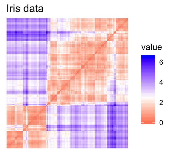
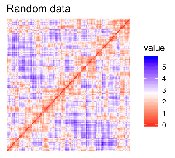
- Red: high similarity (ie: low dissimilarity) | Blue: low similarity
The color level is proportional to the value of the dissimilarity between observations: pure red if \(dist(x_i, x_j) = 0\) and pure blue if \(dist(x_i, x_j) = 1\). Objects belonging to the same cluster are displayed in consecutive order.
The dissimilarity matrix image confirms that there is a cluster structure in the iris data set but not in the random one.
The VAT detects the clustering tendency in a visual form by counting the number of square shaped dark blocks along the diagonal in a VAT image.
Summary
In this article, we described how to assess clustering tendency using the Hopkins statistics and a visual method. After showing that a data is clusterable, the next step is to determine the number of optimal clusters in the data. This will be described in the next chapter.
References
Han, Jiawei, Micheline Kamber, and Jian Pei. 2012. Data Mining: Concepts and Techniques. 3rd ed. Boston: Morgan Kaufmann. https://doi.org/10.1016/B978-0-12-381479-1.00016-2.
Lawson, Richard G., and Peter C. Jurs. 1990. “New Index for Clustering Tendency and Its Application to Chemical Problems.” Journal of Chemical Information and Computer Sciences 30 (1): 36–41. http://pubs.acs.org/doi/abs/10.1021/ci00065a010.
Recommended for you
This section contains best data science and self-development resources to help you on your path.
Coursera - Online Courses and Specialization
Data science
- Course: Machine Learning: Master the Fundamentals by Stanford
- Specialization: Data Science by Johns Hopkins University
- Specialization: Python for Everybody by University of Michigan
- Courses: Build Skills for a Top Job in any Industry by Coursera
- Specialization: Master Machine Learning Fundamentals by University of Washington
- Specialization: Statistics with R by Duke University
- Specialization: Software Development in R by Johns Hopkins University
- Specialization: Genomic Data Science by Johns Hopkins University
Popular Courses Launched in 2020
- Google IT Automation with Python by Google
- AI for Medicine by deeplearning.ai
- Epidemiology in Public Health Practice by Johns Hopkins University
- AWS Fundamentals by Amazon Web Services
Trending Courses
- The Science of Well-Being by Yale University
- Google IT Support Professional by Google
- Python for Everybody by University of Michigan
- IBM Data Science Professional Certificate by IBM
- Business Foundations by University of Pennsylvania
- Introduction to Psychology by Yale University
- Excel Skills for Business by Macquarie University
- Psychological First Aid by Johns Hopkins University
- Graphic Design by Cal Arts
Amazon FBA
Amazing Selling Machine
Books - Data Science
Our Books
- Practical Guide to Cluster Analysis in R by A. Kassambara (Datanovia)
- Practical Guide To Principal Component Methods in R by A. Kassambara (Datanovia)
- Machine Learning Essentials: Practical Guide in R by A. Kassambara (Datanovia)
- R Graphics Essentials for Great Data Visualization by A. Kassambara (Datanovia)
- GGPlot2 Essentials for Great Data Visualization in R by A. Kassambara (Datanovia)
- Network Analysis and Visualization in R by A. Kassambara (Datanovia)
- Practical Statistics in R for Comparing Groups: Numerical Variables by A. Kassambara (Datanovia)
- Inter-Rater Reliability Essentials: Practical Guide in R by A. Kassambara (Datanovia)
Others
- R for Data Science: Import, Tidy, Transform, Visualize, and Model Data by Hadley Wickham & Garrett Grolemund
- Hands-On Machine Learning with Scikit-Learn, Keras, and TensorFlow: Concepts, Tools, and Techniques to Build Intelligent Systems by Aurelien Géron
- Practical Statistics for Data Scientists: 50 Essential Concepts by Peter Bruce & Andrew Bruce
- Hands-On Programming with R: Write Your Own Functions And Simulations by Garrett Grolemund & Hadley Wickham
- An Introduction to Statistical Learning: with Applications in R by Gareth James et al.
- Deep Learning with R by François Chollet & J.J. Allaire
- Deep Learning with Python by François Chollet

Hi,
this is a very nicely written/explained article, thank you for posting!
I am trying to recreate what you did but I got a different result for
`res <- get_clust_tendency(df, n = nrow(df)-1, graph = FALSE)
res$hopkins_stat`
Instead of 0.818 I am getting 0.1815219. I use set.seed(123) and I literally copy paste your code so I can get the same result. No luck! I would appreciate a comment on this! Thank you!
Good day!
Hi,
Thank you for your feedback!
Please, make sure you have install the latest developmental version of factoextra:
devtools::install_github("kassambara/factoextra")Let me know if it works…
https://cran.r-project.org/web/packages/factoextra/factoextra.pdf
it is written below 0.5 is highly clusterable
but in this it is 0.8
how it is highly clusterable
Same thing happening to me. Did you have any luck fixing it?
Please install the latest developmental version of factoextra:
devtools::install_github("kassambara/factoextra")I could be wrong but the code used to generate the Hokin’s statistic appears to produce 1-H. Based on the formula you list
H=∑i=1nyi ∑i=1nxi+∑i=1nyi
The sum of the distances for the artificial points is listed in the nuemerator. However, at the end of the source code for the “get_clust_tendency” function the statistic is calculated as
hopkins_stat = sum(minq)/(sum(minp) + sum(minq))
If I understand the code correctly then ity looks as if “p” is the artificial uniform distributed data
( p <- apply(data, 2,function(x, n) {
runif(n, min(x), max(x))
}, n) )
and "q" should be the random sample of your actually data
k <- round(runif(n, 1, nrow(data)))
q <- as.matrix(data[k, ])
I am also questioning if the get_clust_tendency from devtools::install_github(“kassambara/factoextra”) produces 1-H instead of H.
There is also a discussion here: https://stats.stackexchange.com/questions/332651/validating-cluster-tendency-using-hopkins-statistic
Can the author please confirm?
Please make sure you have the latest developmental version of factoextra, which computes H.
You can install it as follow:
if(!require(devtools)) install.packages("devtools") devtools::install_github("kassambara/factoextra")If v.1.0.5 and beyond computes H, then ;
res = get_clust_tendency(
data = data,
n = nrow(data)-1,
graph = F
)
res$hopkins_stat = 0.1815219
——
Here data is the standardised Iris dataset. How do we proceed?
hi, can we apply the same method to for a mixed data set with categorical or binary variables
For a mixed data, you can, first, compute a distance matrix between variables using the daisy() R function [in cluster package]. Next, you can apply hierarchical clustering on the computed distance matrix.
If you want to use principal component methods on mixed data, see this article:
http://www.sthda.com/english/articles/31-principal-component-methods-in-r-practical-guide/
Hello,
I am trying to install ‘facoextra’ thru devtools and github. it is showing several packages shown below. Which one to choose?
Regards,
1: assertthat (0.2.0 -> 0.2.1 ) [CRAN] 2: cli (1.0.1 -> 1.1.0 ) [CRAN]
3: clipr (0.5.0 -> 0.6.0 ) [CRAN] 4: colorspace (1.4-0 -> 1.4-1 ) [CRAN]
5: data.table (1.12.0 -> 1.12.2) [CRAN] 6: ggplot2 (3.1.0 -> 3.1.1 ) [CRAN]
7: glue (1.3.0 -> 1.3.1 ) [CRAN] 8: gtable (0.2.0 -> 0.3.0 ) [CRAN]
9: lazyeval (0.2.1 -> 0.2.2 ) [CRAN] 10: lme4 (1.1-20 -> 1.1-21) [CRAN]
11: maptools (0.9-4 -> 0.9-5 ) [CRAN] 12: purrr (0.3.0 -> 0.3.2 ) [CRAN]
13: Rcpp (1.0.0 -> 1.0.1 ) [CRAN] 14: readxl (1.3.0 -> 1.3.1 ) [CRAN]
15: rlang (0.3.1 -> 0.3.4 ) [CRAN] 16: stringi (1.3.1 -> 1.4.3 ) [CRAN]
17: tibble (2.0.1 -> 2.1.1 ) [CRAN] 18: CRAN packages only
19: All 20: None
Hi,
R is asking if you want to update old packages. Type 20 in R console to ignore these updates and try.
Hi Kassambara,
Thanks for producing so much useful content! Your website is great.
However, you said in a comment here that the get_clust_tendency() function in version 1.0.5 of ‘factoextra’ generates H, rather than 1 – H. This is incorrect, as far as I can tell, because I am using ‘factoextra’ version 1.0.5, and get output values from get_clust_tendency() which are virtually identical to the output of the hopkins() function from ‘clustertend’ (which, as you know, outputs 1 – H). I have tested this with different datasets, and it seems the get_clust_tendency() function in version 1.0.5 of ‘factoextra’ generates 1 – H, not H.
Please consider providing a proper explanation in the main text of this tutorial, of when and how the get_clust_tendency() function from ‘factoextra’ was changed.
Many people rely on the content of your website, and not providing a proper explanation has resulted in quite a lot of confusion, as you can see from the comments here and discussions elsewhere too: https://stats.stackexchange.com/questions/332651/validating-cluster-tendency-using-hopkins-statistic
Many thanks again for the useful content!
Thank you for your feedback. I updated my previous comment. It is the latest developmental version of factoextra that returns H instead of 1-H (https://github.com/kassambara/factoextra/blob/master/NEWS.md).
You can install it as follow:
if(!require(devtools)) install.packages("devtools")
devtools::install_github("kassambara/factoextra")
I’m submitting it to CRAN now.
Very good. Thanks again! I’m sure future visitors to this page will be grateful for the clarification.
Nice blog!Learn a lot and thanks a lot!
But I still have no idea about how to perform mixed data to obtain the Hopskin statistic.I will really appreciate ,if you can reply.