The agglomerative clustering is the most common type of hierarchical clustering used to group objects in clusters based on their similarity. It’s also known as AGNES (Agglomerative Nesting). The algorithm starts by treating each object as a singleton cluster. Next, pairs of clusters are successively merged until all clusters have been merged into one big cluster containing all objects. The result is a tree-based representation of the objects, named dendrogram.
In this article, we start by describing the agglomerative clustering algorithms. Next, we provide R lab sections with many examples for computing and visualizing hierarchical clustering. We continue by explaining how to interpret dendrogram. Finally, we provide R codes for cutting dendrograms into groups.
Contents:
Related Book
Practical Guide to Cluster Analysis in RAlgorithm
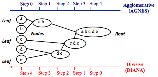
Agglomerative clustering works in a “bottom-up” manner. That is, each object is initially considered as a single-element cluster (leaf). At each step of the algorithm, the two clusters that are the most similar are combined into a new bigger cluster (nodes). This procedure is iterated until all points are member of just one single big cluster (root) (see figure below).
The inverse of agglomerative clustering is divisive clustering, which is also known as DIANA (Divise Analysis) and it works in a “top-down” manner. It begins with the root, in which all objects are included in a single cluster. At each step of iteration, the most heterogeneous cluster is divided into two. The process is iterated until all objects are in their own cluster (see figure below).
Note that, agglomerative clustering is good at identifying small clusters. Divisive clustering is good at identifying large clusters. In this article, we’ll focus mainly on agglomerative hierarchical clustering.
Steps to agglomerative hierarchical clustering
We’ll follow the steps below to perform agglomerative hierarchical clustering using R software:
- Preparing the data
- Computing (dis)similarity information between every pair of objects in the data set.
- Using linkage function to group objects into hierarchical cluster tree, based on the distance information generated at step 1. Objects/clusters that are in close proximity are linked together using the linkage function.
- Determining where to cut the hierarchical tree into clusters. This creates a partition of the data.
We’ll describe each of these steps in the next section.
Data structure and preparation
The data should be a numeric matrix with:
- rows representing observations (individuals);
- and columns representing variables.
Here, we’ll use the R base USArrests data sets.
Note that, it’s generally recommended to standardize variables in the data set before performing subsequent analysis. Standardization makes variables comparable, when they are measured in different scales. For example one variable can measure the height in meter and another variable can measure the weight in kg. The R function scale() can be used for standardization, See ?scale documentation.
# Load the data
data("USArrests")

# Standardize the data
df <- scale(USArrests)

# Show the first 6 rows
head(df, nrow = 6)
## Murder Assault UrbanPop Rape
## Alabama 1.2426 0.783 -0.521 -0.00342
## Alaska 0.5079 1.107 -1.212 2.48420
## Arizona 0.0716 1.479 0.999 1.04288
## Arkansas 0.2323 0.231 -1.074 -0.18492
## California 0.2783 1.263 1.759 2.06782
## Colorado 0.0257 0.399 0.861 1.86497Similarity measures
In order to decide which objects/clusters should be combined or divided, we need methods for measuring the similarity between objects.
There are many methods to calculate the (dis)similarity information, including Euclidean and manhattan distances. In R software, you can use the function dist() to compute the distance between every pair of object in a data set. The results of this computation is known as a distance or dissimilarity matrix.
By default, the function dist() computes the Euclidean distance between objects; however, it’s possible to indicate other metrics using the argument method. See ?dist for more information.
For example, consider the R base data set USArrests, you can compute the distance matrix as follow:
# Compute the dissimilarity matrix
# df = the standardized data
res.dist <- dist(df, method = "euclidean")
Note that, the function dist() computes the distance between the rows of a data matrix using the specified distance measure method.
To see easily the distance information between objects, we reformat the results of the function dist() into a matrix using the as.matrix() function. In this matrix, value in the cell formed by the row i, the column j, represents the distance between object i and object j in the original data set. For instance, element 1,1 represents the distance between object 1 and itself (which is zero). Element 1,2 represents the distance between object 1 and object 2, and so on.
The R code below displays the first 6 rows and columns of the distance matrix:
as.matrix(res.dist)[1:6, 1:6]## Alabama Alaska Arizona Arkansas California Colorado
## Alabama 0.00 2.70 2.29 1.29 3.26 2.65
## Alaska 2.70 0.00 2.70 2.83 3.01 2.33
## Arizona 2.29 2.70 0.00 2.72 1.31 1.37
## Arkansas 1.29 2.83 2.72 0.00 3.76 2.83
## California 3.26 3.01 1.31 3.76 0.00 1.29
## Colorado 2.65 2.33 1.37 2.83 1.29 0.00Linkage
The linkage function takes the distance information, returned by the function dist(), and groups pairs of objects into clusters based on their similarity. Next, these newly formed clusters are linked to each other to create bigger clusters. This process is iterated until all the objects in the original data set are linked together in a hierarchical tree.
For example, given a distance matrix “res.dist” generated by the function dist(), the R base function hclust() can be used to create the hierarchical tree.
hclust() can be used as follow:
res.hc <- hclust(d = res.dist, method = "ward.D2")- d: a dissimilarity structure as produced by the dist() function.
- method: The agglomeration (linkage) method to be used for computing distance between clusters. Allowed values is one of “ward.D”, “ward.D2”, “single”, “complete”, “average”, “mcquitty”, “median” or “centroid”.
There are many cluster agglomeration methods (i.e, linkage methods). The most common linkage methods are described below.
- Maximum or complete linkage: The distance between two clusters is defined as the maximum value of all pairwise distances between the elements in cluster 1 and the elements in cluster 2. It tends to produce more compact clusters.
- Minimum or single linkage: The distance between two clusters is defined as the minimum value of all pairwise distances between the elements in cluster 1 and the elements in cluster 2. It tends to produce long, “loose” clusters.
- Mean or average linkage: The distance between two clusters is defined as the average distance between the elements in cluster 1 and the elements in cluster 2.
- Centroid linkage: The distance between two clusters is defined as the distance between the centroid for cluster 1 (a mean vector of length p variables) and the centroid for cluster 2.
- Ward’s minimum variance method: It minimizes the total within-cluster variance. At each step the pair of clusters with minimum between-cluster distance are merged.
Note that, at each stage of the clustering process the two clusters, that have the smallest linkage distance, are linked together.
Complete linkage and Ward’s method are generally preferred.
Dendrogram
Dendrograms correspond to the graphical representation of the hierarchical tree generated by the function hclust(). Dendrogram can be produced in R using the base function plot(res.hc), where res.hc is the output of hclust(). Here, we’ll use the function fviz_dend()[ in factoextra R package] to produce a beautiful dendrogram.
First install factoextra by typing this: install.packages(“factoextra”); next visualize the dendrogram as follow:
# cex: label size
library("factoextra")
fviz_dend(res.hc, cex = 0.5)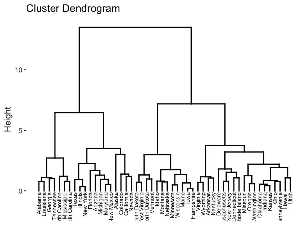
In the dendrogram displayed above, each leaf corresponds to one object. As we move up the tree, objects that are similar to each other are combined into branches, which are themselves fused at a higher height.
The height of the fusion, provided on the vertical axis, indicates the (dis)similarity/distance between two objects/clusters. The higher the height of the fusion, the less similar the objects are. This height is known as the cophenetic distance between the two objects.
Note that, conclusions about the proximity of two objects can be drawn only based on the height where branches containing those two objects first are fused. We cannot use the proximity of two objects along the horizontal axis as a criteria of their similarity.
In order to identify sub-groups, we can cut the dendrogram at a certain height as described in the next sections.
Verify the cluster tree
After linking the objects in a data set into a hierarchical cluster tree, you might want to assess that the distances (i.e., heights) in the tree reflect the original distances accurately.
One way to measure how well the cluster tree generated by the hclust() function reflects your data is to compute the correlation between the cophenetic distances and the original distance data generated by the dist() function. If the clustering is valid, the linking of objects in the cluster tree should have a strong correlation with the distances between objects in the original distance matrix.
The closer the value of the correlation coefficient is to 1, the more accurately the clustering solution reflects your data. Values above 0.75 are felt to be good. The “average” linkage method appears to produce high values of this statistic. This may be one reason that it is so popular.
The R base function cophenetic() can be used to compute the cophenetic distances for hierarchical clustering.
# Compute cophentic distance
res.coph <- cophenetic(res.hc)

# Correlation between cophenetic distance and
# the original distance
cor(res.dist, res.coph)
## [1] 0.698Execute the hclust() function again using the average linkage method. Next, call cophenetic() to evaluate the clustering solution.
res.hc2 <- hclust(res.dist, method = "average")

cor(res.dist, cophenetic(res.hc2))
## [1] 0.718The correlation coefficient shows that using a different linkage method creates a tree that represents the original distances slightly better.
Cut the dendrogram into different groups
One of the problems with hierarchical clustering is that, it does not tell us how many clusters there are, or where to cut the dendrogram to form clusters.
You can cut the hierarchical tree at a given height in order to partition your data into clusters. The R base function cutree() can be used to cut a tree, generated by the hclust() function, into several groups either by specifying the desired number of groups or the cut height. It returns a vector containing the cluster number of each observation.
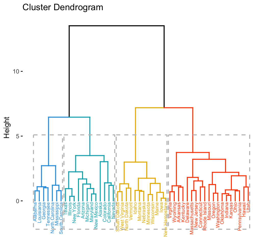
# Cut tree into 4 groups
grp <- cutree(res.hc, k = 4)
head(grp, n = 4)
## Alabama Alaska Arizona Arkansas
## 1 2 2 3# Number of members in each cluster
table(grp)## grp
## 1 2 3 4
## 7 12 19 12# Get the names for the members of cluster 1
rownames(df)[grp == 1]## [1] "Alabama" "Georgia" "Louisiana" "Mississippi"
## [5] "North Carolina" "South Carolina" "Tennessee"The result of the cuts can be visualized easily using the function fviz_dend() [in factoextra]:
Claim Your Membership Now.
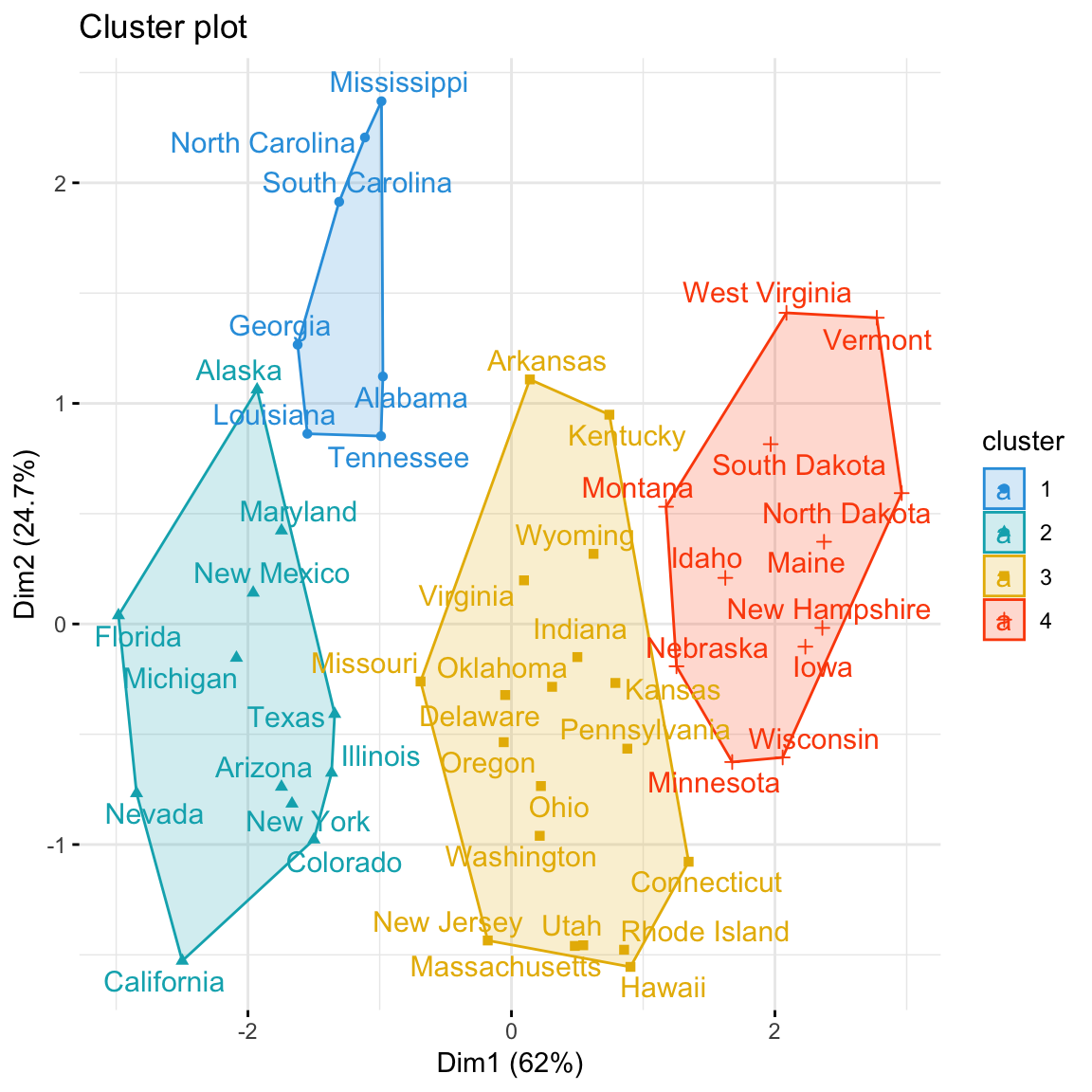
Using the function fviz_cluster() [in factoextra], we can also visualize the result in a scatter plot. Observations are represented by points in the plot, using principal components. A frame is drawn around each cluster.
Claim Your Membership Now.
Cluster R package
The R package cluster makes it easy to perform cluster analysis in R. It provides the function agnes() and diana() for computing agglomerative and divisive clustering, respectively. These functions perform all the necessary steps for you. You don’t need to execute the scale(), dist() and hclust() function separately.
The functions can be executed as follow:
library("cluster")
# Agglomerative Nesting (Hierarchical Clustering)
res.agnes <- agnes(x = USArrests, # data matrix
                   stand = TRUE, # Standardize the data
                   metric = "euclidean", # metric for distance matrix
                   method = "ward" # Linkage method
                   )

# DIvisive ANAlysis Clustering
res.diana <- diana(x = USArrests, # data matrix
                   stand = TRUE, # standardize the data
                   metric = "euclidean" # metric for distance matrix
                   )
After running agnes() and diana(), you can use the function fviz_dend()[in factoextra] to visualize the output:
fviz_dend(res.agnes, cex = 0.6, k = 4)Application of hierarchical clustering to gene expression data analysis
In gene expression data analysis, clustering is generaly used as one of the first step to explore the data. We are interested in whether there are groups of genes or groups of samples that have similar gene expression patterns.
Several clustering distance measures have been described for assessing the similarity or the dissimilarity between items, in order to decide which items have to be grouped together or not. These measures can be used to cluster genes or samples that are similar.
For most common clustering softwares, the default distance measure is the Euclidean distance. The most popular methods for gene expression data are to use log2(expression + 0.25), correlation distance and complete linkage clustering agglomerative-clustering.
Single and Complete linkage give the same dendrogram whether you use the raw data, the log of the data or any other transformation of the data that preserves the order because what matters is which ones have the smallest distance. The other methods are sensitive to the measurement scale.
Note that, when the data are scaled, the Euclidean distance of the z-scores is the same as correlation distance.
Pearson’s correlation is quite sensitive to outliers. When clustering genes, it is important to be aware of the possible impact of outliers. An alternative option is to use Spearman’s correlation instead of Pearson’s correlation.
In principle it is possible to cluster all the genes, although visualizing a huge dendrogram might be problematic. Usually, some type of preliminary analysis, such as differential expression analysis is used to select genes for clustering.
Selecting genes based on differential expression analysis removes genes which are likely to have only chance patterns. This should enhance the patterns found in the gene clusters.
Summary
Hierarchical clustering is a cluster analysis method, which produce a tree-based representation (i.e.: dendrogram) of a data. Objects in the dendrogram are linked together based on their similarity.
To perform hierarchical cluster analysis in R, the first step is to calculate the pairwise distance matrix using the function dist(). Next, the result of this computation is used by the hclust() function to produce the hierarchical tree. Finally, you can use the function fviz_dend() [in factoextra R package] to plot easily a beautiful dendrogram.
It’s also possible to cut the tree at a given height for partitioning the data into multiple groups (R function cutree()).
Recommended for you
This section contains best data science and self-development resources to help you on your path.
Coursera - Online Courses and Specialization
Data science
- Course: Machine Learning: Master the Fundamentals by Stanford
- Specialization: Data Science by Johns Hopkins University
- Specialization: Python for Everybody by University of Michigan
- Courses: Build Skills for a Top Job in any Industry by Coursera
- Specialization: Master Machine Learning Fundamentals by University of Washington
- Specialization: Statistics with R by Duke University
- Specialization: Software Development in R by Johns Hopkins University
- Specialization: Genomic Data Science by Johns Hopkins University
Popular Courses Launched in 2020
- Google IT Automation with Python by Google
- AI for Medicine by deeplearning.ai
- Epidemiology in Public Health Practice by Johns Hopkins University
- AWS Fundamentals by Amazon Web Services
Trending Courses
- The Science of Well-Being by Yale University
- Google IT Support Professional by Google
- Python for Everybody by University of Michigan
- IBM Data Science Professional Certificate by IBM
- Business Foundations by University of Pennsylvania
- Introduction to Psychology by Yale University
- Excel Skills for Business by Macquarie University
- Psychological First Aid by Johns Hopkins University
- Graphic Design by Cal Arts
Amazon FBA
Amazing Selling Machine
Books - Data Science
Our Books
- Practical Guide to Cluster Analysis in R by A. Kassambara (Datanovia)
- Practical Guide To Principal Component Methods in R by A. Kassambara (Datanovia)
- Machine Learning Essentials: Practical Guide in R by A. Kassambara (Datanovia)
- R Graphics Essentials for Great Data Visualization by A. Kassambara (Datanovia)
- GGPlot2 Essentials for Great Data Visualization in R by A. Kassambara (Datanovia)
- Network Analysis and Visualization in R by A. Kassambara (Datanovia)
- Practical Statistics in R for Comparing Groups: Numerical Variables by A. Kassambara (Datanovia)
- Inter-Rater Reliability Essentials: Practical Guide in R by A. Kassambara (Datanovia)
Others
- R for Data Science: Import, Tidy, Transform, Visualize, and Model Data by Hadley Wickham & Garrett Grolemund
- Hands-On Machine Learning with Scikit-Learn, Keras, and TensorFlow: Concepts, Tools, and Techniques to Build Intelligent Systems by Aurelien Géron
- Practical Statistics for Data Scientists: 50 Essential Concepts by Peter Bruce & Andrew Bruce
- Hands-On Programming with R: Write Your Own Functions And Simulations by Garrett Grolemund & Hadley Wickham
- An Introduction to Statistical Learning: with Applications in R by Gareth James et al.
- Deep Learning with R by François Chollet & J.J. Allaire
- Deep Learning with Python by François Chollet

This article is amazing! It’s simply, but skillfully written and easy to fallow. Can’t wait to read new one!
P.S. I started loving my internship at bioinformatics lab even more now. Keep doing your mojo! 🙂
Thank you Jovana for this positive feedback, highly appreciated!
Im not sure if I understand the output of the Scatterplot. We obviously have all the clusters, however, I cant seem to figure out what the percentages along the X and Y axis represents.
Are these the the fractions of the total variation in the data, that the clusters captures along each dimension?
The percentage is the variation of distance and it’s in 2 dimensions. What you seeing is about 86% of the total distance between each point in each cluster, in a two dimension plot. If you add one more dimension it will increase
Hey, thank you for your support. I wanted to color the labels based on the grouping they originally from and color the branches based on the new clustering. can you please help?
Hi, I want to try the code on my computer. Do I need to go somewhere download the data set USArrests.csv?