The k-medoids algorithm is a clustering approach related to k-means clustering for partitioning a data set into k groups or clusters. In k-medoids clustering, each cluster is represented by one of the data point in the cluster. These points are named cluster medoids.
The term medoid refers to an object within a cluster for which average dissimilarity between it and all the other the members of the cluster is minimal. It corresponds to the most centrally located point in the cluster. These objects (one per cluster) can be considered as a representative example of the members of that cluster which may be useful in some situations. Recall that, in k-means clustering, the center of a given cluster is calculated as the mean value of all the data points in the cluster.
K-medoid is a robust alternative to k-means clustering. This means that, the algorithm is less sensitive to noise and outliers, compared to k-means, because it uses medoids as cluster centers instead of means (used in k-means).
The k-medoids algorithm requires the user to specify k, the number of clusters to be generated (like in k-means clustering). A useful approach to determine the optimal number of clusters is the silhouette method, described in the next sections.
The most common k-medoids clustering methods is the PAM algorithm (Partitioning Around Medoids, (Kaufman and Rousseeuw 1990)).
In this article, We’ll describe the PAM algorithm and show how to compute PAM in R software.
In the next article, we’ll also discuss a variant of PAM named CLARA (Clustering Large Applications) which is used for analyzing large data sets.
Contents:
Related Book
Practical Guide to Cluster Analysis in RPAM concept
The use of means implies that k-means clustering is highly sensitive to outliers. This can severely affects the assignment of observations to clusters. A more robust algorithm is provided by the PAM algorithm.
PAM algorithm
The PAM algorithm is based on the search for k representative objects or medoids among the observations of the data set.
After finding a set of k medoids, clusters are constructed by assigning each observation to the nearest medoid.
Next, each selected medoid m and each non-medoid data point are swapped and the objective function is computed. The objective function corresponds to the sum of the dissimilarities of all objects to their nearest medoid.
The SWAP step attempts to improve the quality of the clustering by exchanging selected objects (medoids) and non-selected objects. If the objective function can be reduced by interchanging a selected object with an unselected object, then the swap is carried out. This is continued until the objective function can no longer be decreased. The goal is to find k representative objects which minimize the sum of the dissimilarities of the observations to their closest representative object.
In summary, PAM algorithm proceeds in two phases as follow:
Build phase:
- Select k objects to become the medoids, or in case these objects were provided use them as the medoids;
- Calculate the dissimilarity matrix if it was not provided;
- Assign every object to its closest medoid;
Swap phase:
4. For each cluster search if any of the object of the cluster decreases the average dissimilarity coefficient; if it does, select the entity that decreases this coefficient the most as the medoid for this cluster; 5. If at least one medoid has changed go to (3), else end the algorithm.
As mentioned above, the PAM algorithm works with a matrix of dissimilarity, and to compute this matrix the algorithm can use two metrics:
- The euclidean distances, that are the root sum-of-squares of differences;
- And, the Manhattan distance that are the sum of absolute distances.
Note that, in practice, you should get similar results most of the time, using either euclidean or Manhattan distance. If your data contains outliers, Manhattan distance should give more robust results, whereas euclidean would be influenced by unusual values.
Read more on distance measures.
Computing PAM in R
Data
We’ll use the demo data sets “USArrests”, which we start by scaling (Chapter data preparation and R packages) using the R function scale() as follow:
data("USArrests")      # Load the data set
df <- scale(USArrests) # Scale the data
head(df, n = 3)        # View the firt 3 rows of the data
## Murder Assault UrbanPop Rape
## Alabama 1.2426 0.783 -0.521 -0.00342
## Alaska 0.5079 1.107 -1.212 2.48420
## Arizona 0.0716 1.479 0.999 1.04288Required R packages and functions
The function pam() [cluster package] and pamk() [fpc package] can be used to compute PAM.
The function pamk() does not require a user to decide the number of clusters K.
In the following examples, we’ll describe only the function pam(), which simplified format is:
pam(x, k, metric = "euclidean", stand = FALSE)- x: possible values includes:
- Numeric data matrix or numeric data frame: each row corresponds to an observation, and each column corresponds to a variable.
- Dissimilarity matrix: in this case x is typically the output of daisy() or dist()
- k: The number of clusters
- metric: the distance metrics to be used. Available options are “euclidean” and “manhattan”.
- stand: logical value; if true, the variables (columns) in x are standardized before calculating the dissimilarities. Ignored when x is a dissimilarity matrix.
To create a beautiful graph of the clusters generated with the pam() function, will use the factoextra package.
- Installing required packages:
install.packages(c("cluster", "factoextra"))- Loading the packages:
library(cluster)
library(factoextra)
Estimating the optimal number of clusters
To estimate the optimal number of clusters, we’ll use the average silhouette method. The idea is to compute PAM algorithm using different values of clusters k. Next, the average clusters silhouette is drawn according to the number of clusters. The average silhouette measures the quality of a clustering. A high average silhouette width indicates a good clustering. The optimal number of clusters k is the one that maximize the average silhouette over a range of possible values for k (Kaufman and Rousseeuw 1990).
The R function fviz_nbclust() [factoextra package] provides a convenient solution to estimate the optimal number of clusters.
Claim Your Membership Now.
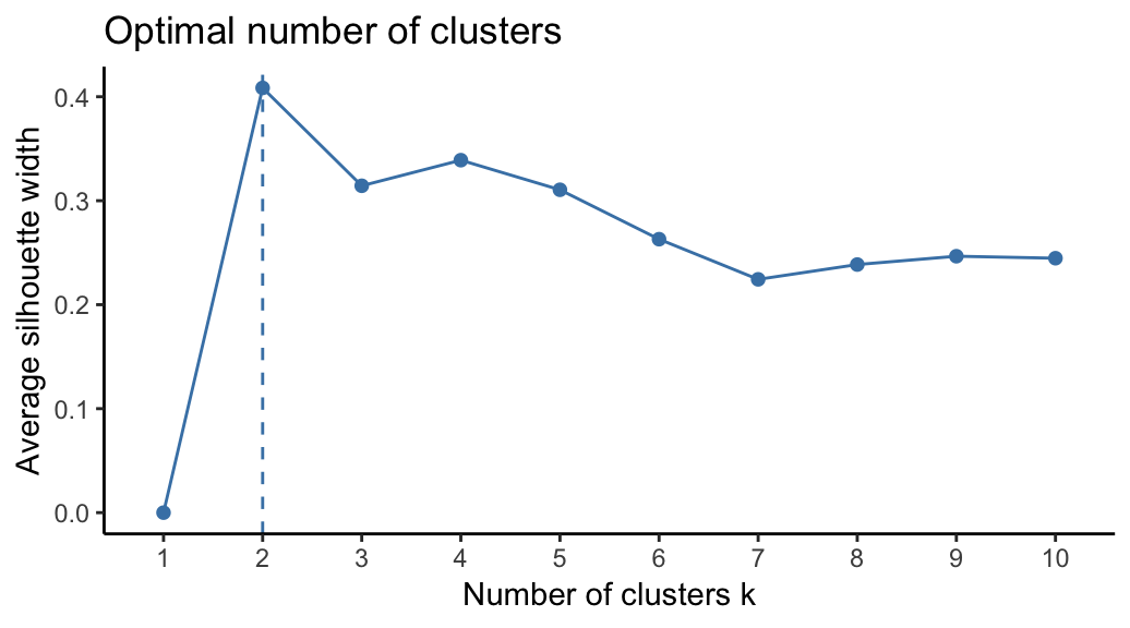
From the plot, the suggested number of clusters is 2. In the next section, we’ll classify the observations into 2 clusters.
Computing PAM clustering
The R code below computes PAM algorithm with k = 2:
pam.res <- pam(df, 2)
print(pam.res)
## Medoids:
## ID Murder Assault UrbanPop Rape
## New Mexico 31 0.829 1.371 0.308 1.160
## Nebraska 27 -0.801 -0.825 -0.245 -0.505
## Clustering vector:
## Alabama Alaska Arizona Arkansas California
## 1 1 1 2 1
## Colorado Connecticut Delaware Florida Georgia
## 1 2 2 1 1
## Hawaii Idaho Illinois Indiana Iowa
## 2 2 1 2 2
## Kansas Kentucky Louisiana Maine Maryland
## 2 2 1 2 1
## Massachusetts Michigan Minnesota Mississippi Missouri
## 2 1 2 1 1
## Montana Nebraska Nevada New Hampshire New Jersey
## 2 2 1 2 2
## New Mexico New York North Carolina North Dakota Ohio
## 1 1 1 2 2
## Oklahoma Oregon Pennsylvania Rhode Island South Carolina
## 2 2 2 2 1
## South Dakota Tennessee Texas Utah Vermont
## 2 1 1 2 2
## Virginia Washington West Virginia Wisconsin Wyoming
## 2 2 2 2 2
## Objective function:
## build swap
## 1.44 1.37
##
## Available components:
## [1] "medoids" "id.med" "clustering" "objective" "isolation"
## [6] "clusinfo" "silinfo" "diss" "call" "data"The printed output shows:
- the cluster medoids: a matrix, which rows are the medoids and columns are variables
- the clustering vector: A vector of integers (from 1:k) indicating the cluster to which each point is allocated
If you want to add the point classifications to the original data, use this:
dd <- cbind(USArrests, cluster = pam.res$cluster)
head(dd, n = 3)
## Murder Assault UrbanPop Rape cluster
## Alabama 13.2 236 58 21.2 1
## Alaska 10.0 263 48 44.5 1
## Arizona 8.1 294 80 31.0 1Accessing to the results of the pam() function
The function pam() returns an object of class pam which components include:
- medoids: Objects that represent clusters
- clustering: a vector containing the cluster number of each object
These components can be accessed as follow:
# Cluster medoids: New Mexico, Nebraska
pam.res$medoids
## Murder Assault UrbanPop Rape
## New Mexico 0.829 1.371 0.308 1.160
## Nebraska -0.801 -0.825 -0.245 -0.505# Cluster numbers
head(pam.res$clustering)## Alabama Alaska Arizona Arkansas California Colorado
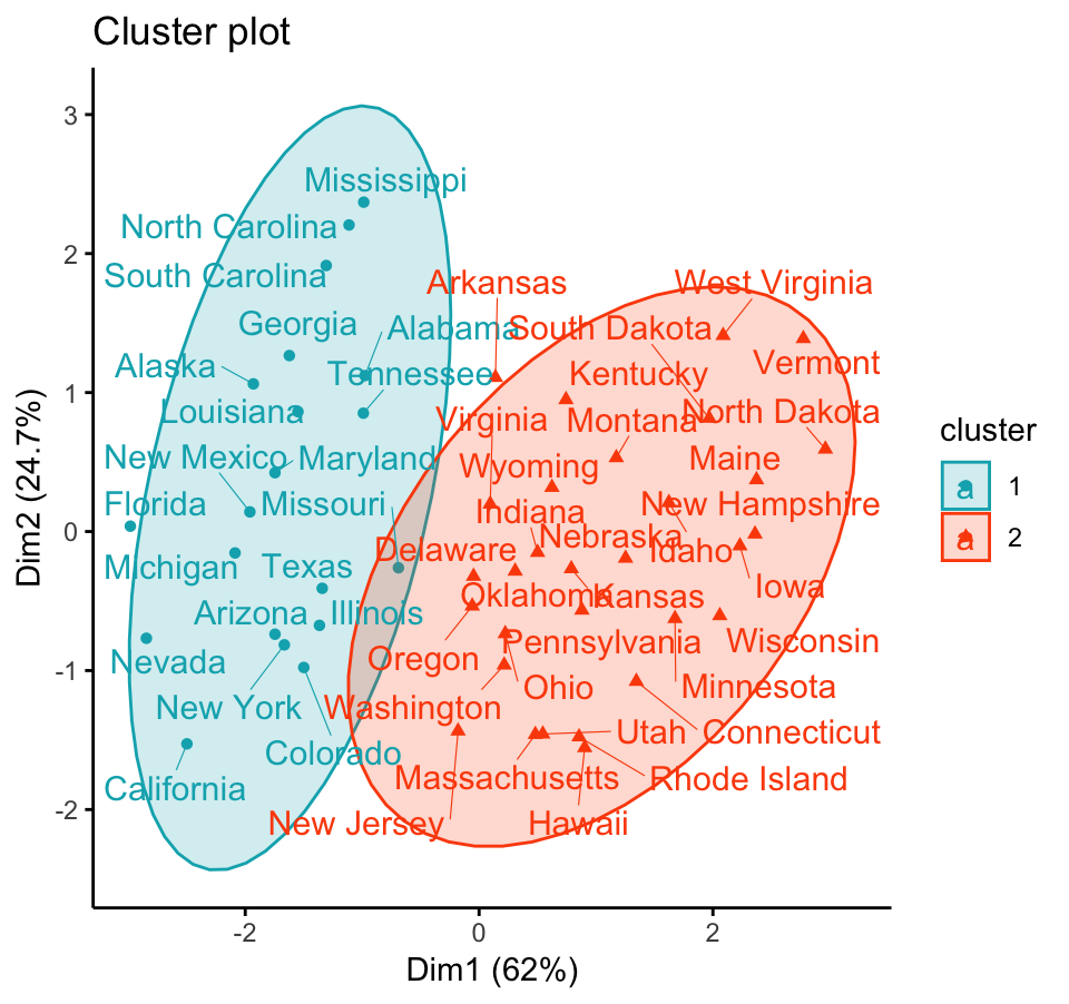
## 1 1 1 2 1 1Visualizing PAM clusters
To visualize the partitioning results, we’ll use the function fviz_cluster() [factoextra package]. It draws a scatter plot of data points colored by cluster numbers. If the data contains more than 2 variables, the Principal Component Analysis (PCA) algorithm is used to reduce the dimensionality of the data. In this case, the first two principal dimensions are used to plot the data.
Claim Your Membership Now.
Summary
The K-medoids algorithm, PAM, is a robust alternative to k-means for partitioning a data set into clusters of observation.
In k-medoids method, each cluster is represented by a selected object within the cluster. The selected objects are named medoids and corresponds to the most centrally located points within the cluster.
The PAM algorithm requires the user to know the data and to indicate the appropriate number of clusters to be produced. This can be estimated using the function fviz_nbclust [in factoextra R package].
The R function pam() [cluster package] can be used to compute PAM algorithm. The simplified format is pam(x, k), where “x” is the data and k is the number of clusters to be generated.
After, performing PAM clustering, the R function fviz_cluster() [factoextra package] can be used to visualize the results. The format is fviz_cluster(pam.res), where pam.res is the PAM results.
Note that, for large data sets, pam() may need too much memory or too much computation time. In this case, the function clara() is preferable. This should not be a problem for modern computers.
References
Kaufman, Leonard, and Peter Rousseeuw. 1990. Finding Groups in Data: An Introduction to Cluster Analysis.
Recommended for you
This section contains best data science and self-development resources to help you on your path.
Coursera - Online Courses and Specialization
Data science
- Course: Machine Learning: Master the Fundamentals by Stanford
- Specialization: Data Science by Johns Hopkins University
- Specialization: Python for Everybody by University of Michigan
- Courses: Build Skills for a Top Job in any Industry by Coursera
- Specialization: Master Machine Learning Fundamentals by University of Washington
- Specialization: Statistics with R by Duke University
- Specialization: Software Development in R by Johns Hopkins University
- Specialization: Genomic Data Science by Johns Hopkins University
Popular Courses Launched in 2020
- Google IT Automation with Python by Google
- AI for Medicine by deeplearning.ai
- Epidemiology in Public Health Practice by Johns Hopkins University
- AWS Fundamentals by Amazon Web Services
Trending Courses
- The Science of Well-Being by Yale University
- Google IT Support Professional by Google
- Python for Everybody by University of Michigan
- IBM Data Science Professional Certificate by IBM
- Business Foundations by University of Pennsylvania
- Introduction to Psychology by Yale University
- Excel Skills for Business by Macquarie University
- Psychological First Aid by Johns Hopkins University
- Graphic Design by Cal Arts
Amazon FBA
Amazing Selling Machine
Books - Data Science
Our Books
- Practical Guide to Cluster Analysis in R by A. Kassambara (Datanovia)
- Practical Guide To Principal Component Methods in R by A. Kassambara (Datanovia)
- Machine Learning Essentials: Practical Guide in R by A. Kassambara (Datanovia)
- R Graphics Essentials for Great Data Visualization by A. Kassambara (Datanovia)
- GGPlot2 Essentials for Great Data Visualization in R by A. Kassambara (Datanovia)
- Network Analysis and Visualization in R by A. Kassambara (Datanovia)
- Practical Statistics in R for Comparing Groups: Numerical Variables by A. Kassambara (Datanovia)
- Inter-Rater Reliability Essentials: Practical Guide in R by A. Kassambara (Datanovia)
Others
- R for Data Science: Import, Tidy, Transform, Visualize, and Model Data by Hadley Wickham & Garrett Grolemund
- Hands-On Machine Learning with Scikit-Learn, Keras, and TensorFlow: Concepts, Tools, and Techniques to Build Intelligent Systems by Aurelien Géron
- Practical Statistics for Data Scientists: 50 Essential Concepts by Peter Bruce & Andrew Bruce
- Hands-On Programming with R: Write Your Own Functions And Simulations by Garrett Grolemund & Hadley Wickham
- An Introduction to Statistical Learning: with Applications in R by Gareth James et al.
- Deep Learning with R by François Chollet & J.J. Allaire
- Deep Learning with Python by François Chollet

Can you plot clusters that have been calculated using distance matrices with pam? I’m trying but I don’t know if the plots are usefull